This section describes how you interface with the main window and its ancillary tools. The primary tools allowing you to load data, analyse, design and apply the Low End and High End operators are described in greater detail in later sections.
The application main window GUI consists of, from top to bottom, a menubar area, a toolbar area, a chart tabs area and a status area (see figure below). The chart tabs area which occupies the large central area of the main window is used to display various charts of spectra and time data providing instant feedback to the Interpretation Geoscientist in his/her quest to design both operators. The four sub-sections which follow will provide you with a description of each of these areas. We will pay particular attention to the central chart area.
This sub-section describes the actions performed by the various menu items.
| Creates a new Frequency Shaping session using the default Broadband Session template (shortcut Ctrl+N). | |
| Creates a new Frequency Shaping session a using a user saved template. By default, the software will look for templates stored in a special directory, created for this purpose, within the application installation tree. | |
| Opens a previously saved Frequency Shaping session (shortcut Ctrl+O). This facility allows you to restore the Frequency Shaping parameters together with the data from a previously saved session. Restoring a previously saved session can take a few moments while database access is established. Note, if the stored data within the database has been modified since the session save time, then it is possible that both operators, which are different to those available at the session save time, might be generated following a session restore. | |
| Saves a Frequency Shaping session. This allows the Frequency Shaping parameters, together with information about the data used, to be saved. In this way, data can be easily reloaded and both operators can be generated at some future date. If this is the first time that this is saved then the user will be presented with a file selector dialog for this purpose (shortcut Ctrl+S). | |
| Saves the current Frequency Shaping session under a different name. A file selector dialog will pop-up for this purpose. See "Save" above for more details. | |
| Saves the current Frequency Shaping session as a new template. By default, new templates will be saved in the site wide templates directory in the software installation tree $CLS_APP/SeisBB/templates/%%templatedir%%. | |
| Saves the Low End and High End operators set to the database. This menu item will pop up a Save Operator dialog. The dialog will list all the operator sets currently stored in the OpendTect database. A filter facility is provided to help you find an existing operator set should your list be very long. Through this dialog you can either select an existing operator set or specify a new database name to save the current operators set. A set will consist of four wavelets with the database name being suffixed with %%_lo%% for the Low End operator, %%_hi%% for the High End operator and %%_lo_bp%% and %%_hi_bp%% for the Low End and High End Band Pass operators. When the Inversion template is used the operators are suffixed %%_sb%% for Spectral Blueing, %%_ci%% for coloured Inversion, and %%_sb_bp%% and %%_ci_bp%% respectively for the spectral blueing and coloured inversion Band Pass operators. | |
The Print option prints both the report and the charts to a specified printer. Alternatively, you can print to file. However, if this option is selected then there is a known bug which will cause the charts output to overwrite the report output. If you need to output both the report and the chart to a file, then use Print Report... and Print Charts... separately. The Print Report... option prints the report to a specified printer. Alternatively, you can print the report to a file. The Print Charts... option prints the charts to a specified printer. Alternatively, you can print the charts to a file. | |
The All Charts... option saves all charts in the central area to an image file. The following image formats are supported: PNG (default) and BMP. The Visible Charts... option saves charts that are currently visible in the central area. | |
The Import Chart Configuration... option pops up a file selector dialog which will allow you to select a previously saved session. The chart configuration of that session file is applied to your current session. Note the data and parameters stored in the session files are ignored. This provides you with a very powerful facility which allows you to view your current data using a variety of different chart configurations. The Export Operator... option allows you to export the operator to an ASCII file. The Export Data Item... option exports one or more of any of the currently displayed data items to an ASCII file. The Import Data Item... option allows you to import from an ASCII file previously exported data items. Only raw data items are imported with this facility. | |
| Pops up a dialog which displays various Frequency Shaping parameters nicely formatted. | |
| Exits the application. |
| Sets the application into Broadband Mode to perform a Low End and High End frequency analysis. The two analysis are performed simultaneously from a single set of parameters | |
| Sets the application into Inversion Mode to perform Coloured Inversion and Spectral Blueing analysis. The two analysis are performed simultaneously from a single set of parameters. The final outputs are two complementary cubes where the peaks on one line up with the zero-crossings on the other. |
| Pops up the "Tabs Controller Dialog" which will allow you to modify each charts tab configuration as well as chart parameters within the central area of the main window. | |
| Redraws all the charts within the current charts tab area. | |
| Provides a global zoom-in facility which makes the current charts tab area grow by a fixed amount each time this menu item is clicked. There is an upper maximum. | |
| Provides a global zoom-out facility which makes the current charts tab area shrink by a fixed amount each time this menu item is clicked. There is a lower minimum. | |
| Provides a seismic view facility that allows the rapid viewing of the input seismic volume. This enables the user to see the effect that the current operator will have in real time. |
| Pops up the "Select Input Data" dialog which allows you to select the seismic and well log data to use in the analysis and operator design. | |
| Pops up the "Design Operator" dialog which allows you to control standard parameters in the design of the Low End and High End operators. | |
| Pops up the tab "Frequency Domain" within the "Advance Controls" dialog which allows you to override many of the frequency domain parameters in the design of both operators. | |
| Pops up the tab "Time Domain" within the "Advance Controls" dialog which allows you to override many of the time domain parameters in the design of both operators. | |
| Pops up the tab "Design Operator" within the "Advance Controls" dialog which allows you to override many of the design operator parameters in the design of both operators. | |
| Pops up the "Well Logs Information" dialog which gives information on the well logs. For each selected well it lists the Low-End and High-End (or Inversion and Blueing) correlation coefficients between a synthetic trace created by convolving the AI log with the Band-Pass filter and the seismic trace at the well location. The Curve Fit alpha and beta values are also listed. | |
| Pops up the "Parameter Test" dialog which allows the testing of a range of Design Operator values in a fast and efficient way. | |
| Pops up the "Time Variant" dialog which allows you to apply operators classified as zones with varying slopes on the seismic data. | |
| Pops up the "Apply Operator" dialog which allows you to apply the operators to the input seismic volume. |
| Pops up an HTML browser displaying the Quick Start document. | |
| Pops up an HTML browser displaying Contents page for software user guide. | |
| Pops up an HTML browser displaying Background and Theory to the software. | |
| Pops up the Application Disgnostics window that allows the level of detail and output destination of diagnostics to be set. If the application behaves in an unexpected way the Application Diagnostics captures the program activity which can help the ARK CLS support staff in determining what is happening. The application should be restarted, ideally from scratch, and the Application Diagnostics turned on before anything else is done. Then the application is run up to the point the problem occures. The diagnostics should then be emailed to support@arkcls.com. | |
| Pops up a file selector dialog allowing you to specify a file which will be used to save information about this installation. The file will be saved as a gzipped compressed text file. ARK CLS support staff may ask you to generate a report to help them resolve issues with the software. If requested, please email this file to support@arkcls.com . | |
| Pops up an HTML browser displaying the home page of ARK CLS Limited website. | |
| Opens a browser window where all our instructional videos are located. There is at least one video dedicated to the SNP application. Alternately, in a browser window, navigate to www.arkcls.com/library/videos | |
| Pops up the About Frequency Shaping window. |
This sub-section describes the actions performed by the various toolbars and their icons. The toolbars can be positioned in various locations within the main window top (default beneath the menu bar), left, right and bottom (above status area). Additionally, the toolbars can be moved off the main window altogether and anchored on the desktop. To move the toolbar to a new location grab the handle at one end of the toolbar by pressing and holding mouse button 1 and dragging to the new location.
 | Sets the application into Broadband Mode to perform a Low End and High End frequency analysis. The two analysis are performed simultaneously from a single set of parameters |
 | Sets the application into Inversion Mode to perform Coloured Inversion and Spectral Blueing analysis. The two analysis are performed simultaneously from a single set of parameters. The final outputs are two complementary cubes where the peaks on one line up with the zero-crossings on the other. |
 | Creates a new Frequency Shaping session. |
 | Opens a previously saved Frequency Shaping session. This facility allows you to restore the Frequency Shaping parameters together with the data from a previously saved session. Restoring a previously saved session can take a few moments while database access is established. Note, if the stored data within the database has been modified since the session save time, then it is possible that both operators, which are different to those available at the session save time, might be generated following a session restore. |
 | Saves a Frequency Shaping session. This allows the Frequency Shaping parameters, together with information about the data used, to be saved. In this way, data can be easily reloaded and both operators generated at some future date. If this is the first time that this is saved then the user will be presented with a file selector dialog for this purpose. |
 | Saves the Frequency Shaping operators set to the database. This menu item will pop up a Save Operator dialog. The dialog will list all the operator sets currently stored in the OpendTect database. A filter facility is provided to help you find an existing operator set should your list be very long. Through this dialog you can either select an existing operator set or specify a new database name to save the current Seismic Broadbnad operator set. A set will consist of four wavelets with the database name being suffixed with %%_lo%% for the Low End operator, %%_hi%% for the High End operator and %%_lo_bp%% and %%_hi_bp%% for the Low End and High End Band Pass operators. |
 | Print both the report and the charts to a specified printer. Alternatively, you can print to file. However, if this option is selected then there is a known bug which will cause the charts to overwrite the report. If you need to output both the report and the chart to a file then use menu File->Print->Print Report... and File->Print->Print Charts... separately. |
 | Displays parameter report. This icon pops up the "Parameter Report" dialog. |
 | Pops up the "Select Input Data" dialog which allows you to select the seismic and well log data to use in the analysis and operator design. |
 | Pops up the "Design Operator" dialog which allows you to control standard parameters in the design of the Low End and High End operators. |
 | Pops up the tab "Frequency Domain" within the "Advance Controls" dialog which allows you to override many of the frequency domain parameters in the design of both operators. |
 | Pops up the tab "Time Domain" within the "Advance Controls" dialog which allows you to override many of the time domain parameters in the design of both operators. |
 | Pops up the tab "Design Operator" within the "Advance Controls" dialog which allows you to override many of the design operator parameters in the design of both operators. |
 | Pops up the "Well Logs Information" dialog which gives information on the well logs. For each selected well it lists the Low-End and High-End (or Inversion and Blueing) correlation coefficients between a synthetic trace created by convolving the AI log with the Band-Pass filter and the seismic trace at the well location. The Curve Fit alpha and beta values are also listed. |
 | Pops up the "Parameter Test" dialog which allows the testing of a range of Design Operator values in a fast and efficient way. |
 | Pops up the "Time Variant" dialog which allows you to apply operators classified as zones with varying slopes on the seismic data. |
 | Pops up the "Apply Operator" dialog which allows you to apply the operators to the input seismic volume. |
 | Pops up the "Tabs Controller Dialog" which will allow you to modify each charts tab configuration as well as chart parameters within the central area of the main window. |
 | Redraws all the charts within the current charts tab area. |
 | Provides a global zoom-in facility which makes the current charts tab area grow by a fixed amount each time this menu item is clicked. There is an upper maximum. |
 | Provides a global zoom-out facility which makes the current charts tab area shrink by a fixed amount each time this menu item is clicked. There is a lower minimum. |
 | Provides a seismic view facility that allows the rapid viewing of the input seismic volume. This enables the user to see the effect that the current operator will have in real time. |
 | This icon pops up the online help system. |
This is the main functional area of the Frequency Shaping application. It is used to display various charts. These charts are used to display various spectra data and time domain data. The chart area provides graphical feedback of the various stages in the generation of the Low End and High End operators for the given data and program parameters supplied by you. The chart area is also dynamic, allowing you to interface directly with the charts within this area. You can interactively update these charts in real time by modifying the various parameters in the "Select Input Data" dialog, "Design Operator" dialog and the "Advanced Controls" dialog. We call this data driven, as the effect of you modifying a parameter within the above dialogs is an immediate update to the graphical charts.
The chart area is highly configurable allowing you to tailor this area with charts and data which meet your particular project needs. Once you have configured this area it can then be saved as a session, which will allow you to easily return to the chart/data configuration at some future date. You can also save the chart area configuration with types of data object to be displayed in a given chart as a template. This will allow you or your colleagues to use such templates on other projects. Another benefit of saving as a template and/or session is that you can apply the chart configuration from a saved template or session to your current session.
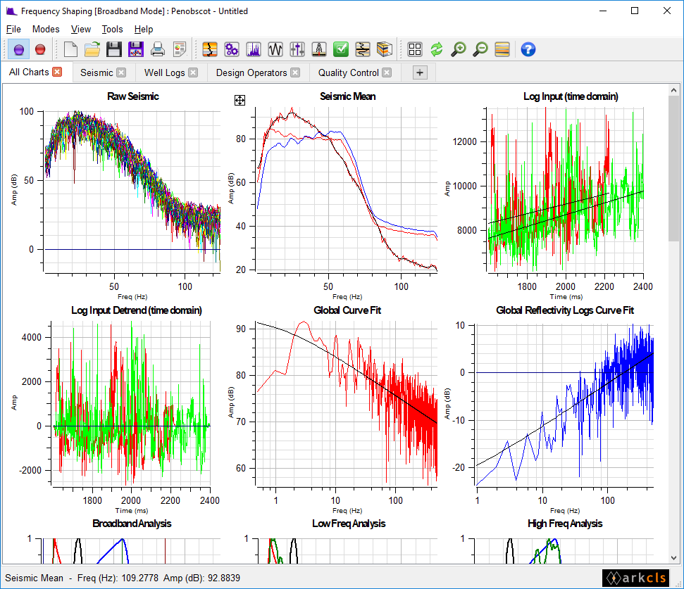
The following figures show an example of a Frequency Shaping run using the supplied default template:
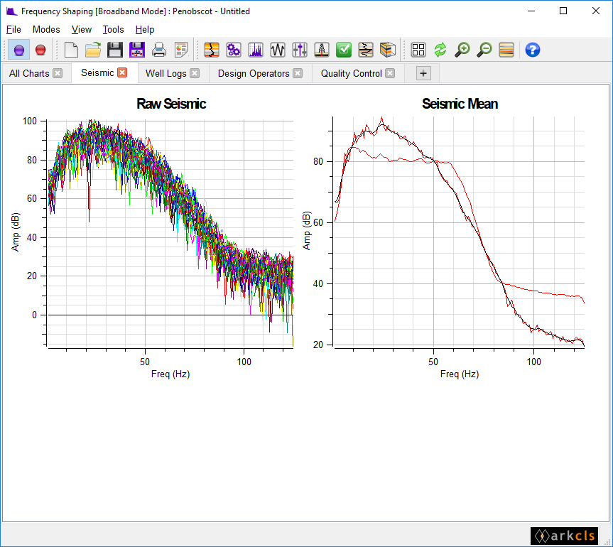
Raw Seismic - This chart displays the raw gated seismic trace spectra. By default, a random set of 40 seismic traces within the 3D Survey Area is loaded when the Load Seismic push button is clicked. This push button is located within the "Input Seismic" tab on the "Select Input Data" dialog. Changing the time gate and/or range mode will update this chart. It is recommended that, if an interpreted horizon (with few undefines) is available within the target area then Range mode (radio button) be set to "Horizon".
Seismic Mean - This chart displays the mean seismic spectrum. The mean seismic spectrum (red) is derived from the raw gated seismic trace spectra in chart 1. Clicking the Load Seismic button within the "Input Seismic" tab on the "Select Input Data Dialog" will update the data on this chart. Also displayed on this chart is a smooth mean seismic spectrum (black). The amount of smoothing can be controlled by you interacting with the Smooth Seismic Mean control on the "Design Operator Dialog".
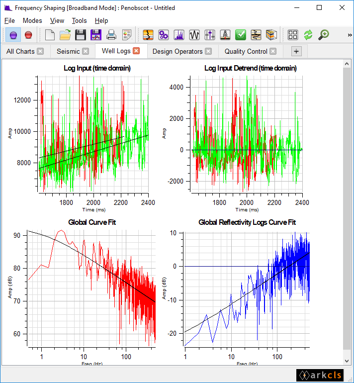
Log Input (time domain) - This chart displays the selected gated AI log data in time. In this example only one AI log has been selected. Selecting or de-selecting AI log data in the "Input Well Log" tab on the "Select Input Data Dialog" will update the data on this chart. Also displayed on this chart is the linear trend line (black). Controls on the "Advanced Controls" dialog can also have an immediate effect on this chart.
Log Input Detrend (time domain) - This chart displays the selected gated AI log data in time with the linear trend line removed. In this case, end ramping has also been applied so the log ends intercept the zero axis. Selecting or de-selecting AI log data in the "Input Well Log" tab on the "Select Input Data Dialog" will update the data on this chart. Controls on the "Advanced Controls" dialog can also have an immediate effect on this chart.
Global Curve Fit - This chart displays the mean (or global) of the individual AI log spectra. In this example, there is only one individual AI log spectrum so the global spectrum is the same as the single individual AI log spectrum. Also displayed on this chart is the curve fit spectrum (black). Various controls on the "Design Operator" dialog and in the "Advanced Controls" dialog can have an immediate effect on this chart.
Global Reflectivity Logs Curve Fit - This chart displays the mean (or global) of the individual AI log spectra. In this example, there is only one individual AI log spectrum so the global spectrum is the same as the single individual AI log spectrum. Also displayed on this chart is the curve fit spectrum (black). Various controls on the "Design Operator" dialog and in the "Advanced Controls" dialog can have an immediate effect on this chart.
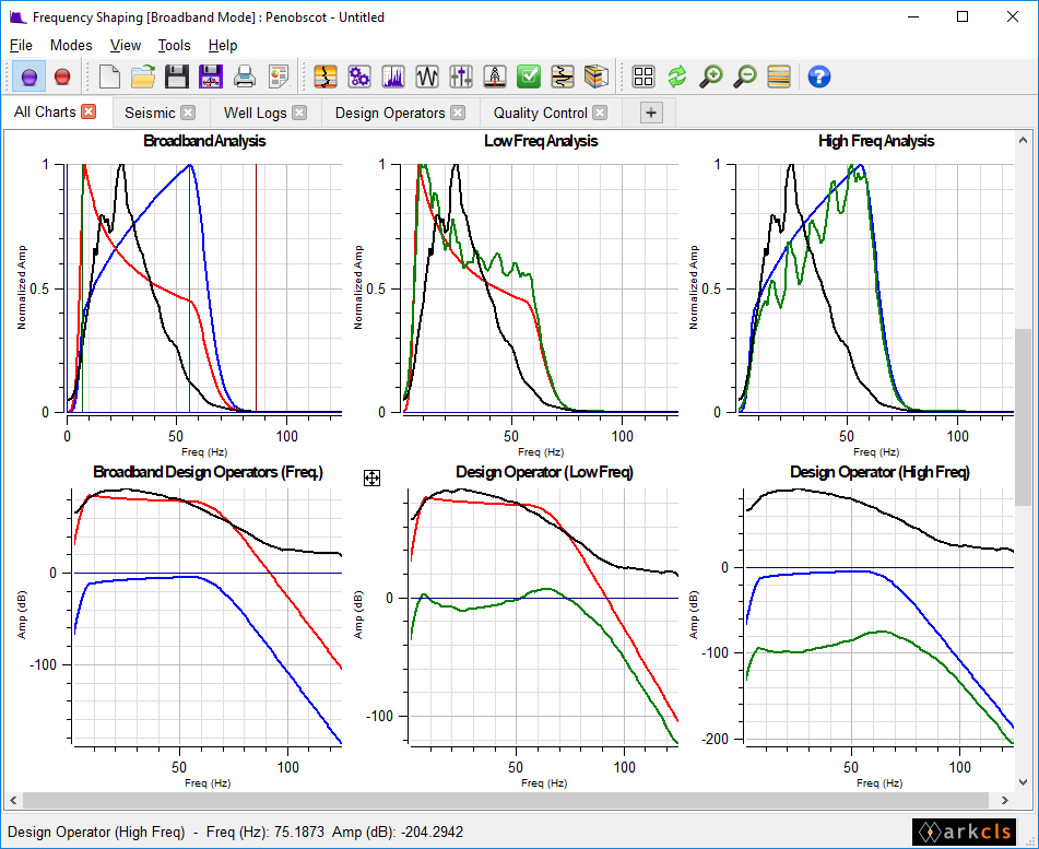
Broadband Analysis - This chart displays a normalized amplitude spectrum of the follow three curves: The curve coloured "black" is the smooth average input seismic. The "red" curve is the band-limited spectrum derived from the smooth composite curve fit to the average AI spectrum. The "blue" curve is the band-limited spectrum derived from the smooth composite curve fit to the average AI reflectivity spectrum. Finally, the vertical lines represent frequency corners F1 to F4 to define the Redding and Shaping operators and the horizon dark cyan line is the -60 dBs attenuation that defined F1 and F4. Note that this chart helps define F1 to F4 owing to the normalised scale that allows direct comparison between low and high frequency composite curves against smoothed average input seismic.
Low Freq. Analysis - This chart displays a normalized amplitude spectrum of the follow three curves: The curve coloured "black" is the smooth average input seismic. The "red" curve is the band-limited spectrum derived from the smooth composite curve fit to the average AI spectrum. The "green" curve is the smooth mean of seismic after applying Low Frequency Operator. Finally, the horizon dark cyan line is the -60 dBs attenuation that defined F1 and F4. Note that this low frequency part of the broandband analysis chart includes the smoothed average spectrum of the seismic resulting from the convolution of the input seismic and reddening operator.
High Freq. Analysis - This chart displays a normalized amplitude spectrum of the follow three curves: The curve coloured "black" is the smooth average input seismic. The "blue" curve is the band-limited spectrum derived from the smooth composite curve fit to the average AI reflectivity spectrum. The "green" curve is the smooth mean of seismic after applying High Frequency Operator. Finally, the horizon dark cyan line is the -60 dBs attenuation that defined F1 and F4. Note that this high frequency part of the broandband analysis chart includes the smoothed average spectrum of the seismic resulting from the convolution of the input seismic and shaping operator.
Broadband Design Operators - This chart displays an amplitude spectrum (in dBs) of the follow three curves: The curve coloured "black" is the smooth average input seismic. The "red" curve is the band-limited spectrum derived from the smooth composite curve fit to the average AI spectrum. The "blue" curve is the band-limited spectrum derived from the smooth composite curve fit to the average AI reflectivity spectrum. Finally, the horizon dark cyan line is the -60 dBs attenuation that defined F1 and F4.
Design Operator (Low Freq) - This chart displays three curves: The curve coloured "red" is the smooth mean seismic spectrum. The "green" curve is the band-limited spectrum derived from the smooth composite curve fit to the average AI spectrum. Finally, the "blue" curve is the band-limited shaping operator. Note: the maximum frequency of the chart is determined by the maximum nyquist frequency of either the log data or the seismic data. Various controls on the "Design Operator Dialog" and in the "Advanced Controls" dialog can have an immediate effect on this chart.
Design Operator (High Freq) - This chart displays three curves: The curve coloured "red" is the smooth mean seismic spectrum. The "green" curve is the band-limited spectrum derived from the smooth composite curve fit to the average AI spectrum. Finally, the "blue" curve is the band-limited shaping operator. Note: the maximum frequency of the chart is determined by the maximum nyquist frequency of either the log data or the seismic data. Various controls on the "Design Operator Dialog" and in the "Advanced Controls" dialog can have an immediate effect on this chart.
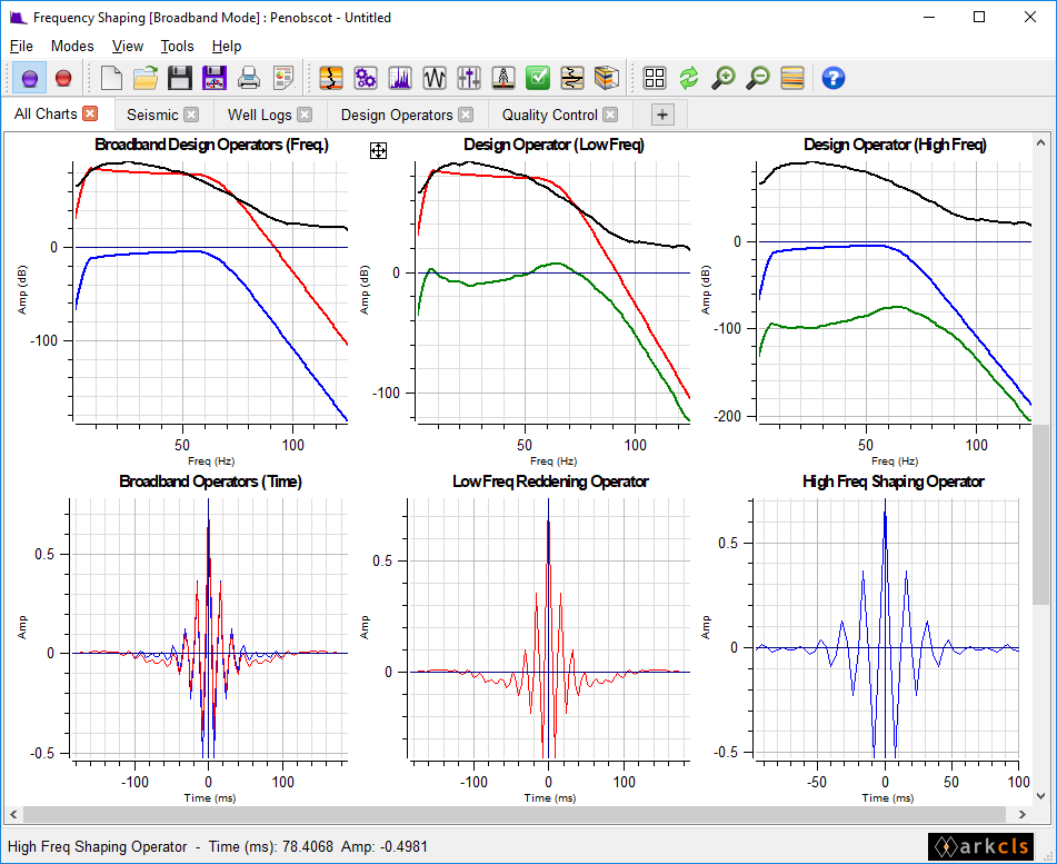
Broadband Operators - This chart displays both the low end and high end operators on the time domain. The curve coloured in red is the Low Frequency operator shape and the curve coloured in blue is the High Frequency operator shape. Various controls in the "Select Input Data" dialog, "Design Operator" dialog and "Advanced Controls" dialog can have an immediate effect on this chart.
Low Freq Reddening Operator - This chart displays the low frequency operator in the time domain. Various controls in the "Select Input Data" dialog, "Design Operator" dialog and "Advanced Controls" dialog can have an immediate effect on this chart.
High Freq Shaping Operator - This chart displays the high frequency operator on the time domain. Various controls in the "Select Input Data" dialog, "Design Operator" dialog and "Advanced Controls" dialog can have an immediate effect on this chart.
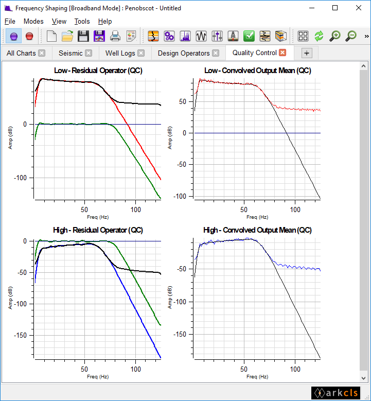
Low - Residual Operator (QC) - This chart displays the following spectra and is used for QC purposes. The black coloured curve is the smooth mean high end seismic data, while the red coloured curve is the band limited curve fit to global AI spectrum and the green coloured curve is the residual low end operator which should tend to be flat and centered around zero.
Low - Convolved Output Mean(QC) - This chart displays the mean Low End data (red) and the smooth mean Low End data (black). Various controls in the "Select Input Data Dialog", "Design Operator Dialog and "Advanced Controls" dialog can have an immediate effect on this chart.
High - Residual Operator (QC) - This chart displays the following spectra and is used for QC purposes. The black coloured curve is the smooth mean high end seismic data, while the blue coloured curve is the band limited curve fit to global AI reflectivity spectrum and the green coloured curve is the residual operator which should tend to be flat and centered around zero.
High - Convolved Output Mean(QC) - This chart displays the mean High End data (blue) and the smooth mean High End data (black). Various controls in the "Select Input Data Dialog", "Design Operator Dialog and "Advanced Controls" dialog can have an immediate effect on this chart.
Various controls in the "Select Input Data" dialog, "Design Operator" dialog and "Advanced Controls" dialog can have an immediate effect on this chart.
The status area at the bottom of the main window is used to display various messages and other information for you. For example, if you pass the mouse over a toolbar icon then a tip is displayed in this area indicating what the purpose of the icon is. The status area is also used to display information about a given chart as the mouse passes over the central area of the main window.
There are various main window ancillary tools within the Frequency Shaping application which you might find helpful and deserve a mention. These are Save Operators, Export Operators, Export Data Items, Import Data Items and Parameter Report.
Clicking the File->Save Operator... menu item in this mode will pop up the "Save Operator" dialog. If you haven't saved the operators during your session or if the operators have changed since you last saved it, then you will be prompted to save the operators before the program exits.
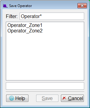
The figure above shows the "Save Operator" dialog. This allows you to select a previously saved low end and high end operators set or to specify a new operators. Either way when you click the Save push button the current time domain operators will be saved to the database by the name in the Select Operator input field here. If the operators already exist in the OpendTect database you will be warned that you are about to overwrite them.
The Import Chart Configuration tool allows you to import from a saved session the chart configuration defined within that session. This is a powerful facility allowing you to rapidly change your display layout using your current data items. Clicking the File->Import/Export...->Import Chart Configuration... menu item will pop up a file selector dialog. Here you can traverse the file system to import the chart configuration from a previously saved session file.
The Export Operator tool allows you to export an operator to an ASCII file. Clicking the File->Import/Export...->Export Operator... menu item will pop up a file selector dialog. Here you can traverse the file system to export both operators as ASCII files.
This is a powerful ancillary tool which allows you to export any of the loaded or generated data items (time or frequency domain curves) to an ASCII file. Clicking the File->Import/Export...->Export Data Items... menu item will pop up the "Export Data Item" dialog.
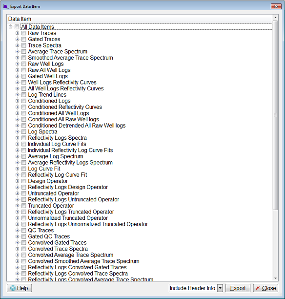
The figure above shows the "Export Data Item" dialog. This dialog contains a list view widget which allows you to export, to an ASCII file, either all the data items for every group, all the data items for a single group or a single data item from a group. This is achieved as follows:
By clicking the "All Data Items" on the "Export Data Item" dialog will select every data item currently available. Then, by clicking the Export push button you will be given a file selector dialog allowing you to save all these data items into a single ASCII file.
By clicking one of the groups beneath the "All Data Items" will select that group. Then, by clicking the Export push button you will again be given a file selector dialog allowing you to save the group data into a single ASCII file.
By clicking a data item within a group will select that data item. Then, by clicking the Export push button you will once again be given a file selector dialog allowing you to save the data item to a single ASCII file.
You can optionally output a header. This is useful if you are outputting two or more data items. It is recommended that you save the session immediately after doing export data items.
This ancillary tool which allows you to import from an ASCII file previously exported data items (see Export Data Item). The only items that are importabled are the raw data items ("Raw Traces", "Raw Well Logs" and "QC Traces") and the "Average Trace Spectrum". All other data items are ignored. By importing the mentioned data items, all derived data items can then be calculated in the normal manner. This tool is particularly useful if a colleague is having problems with software and/or data and has asked you to help but you don't have access to the database where the original seismic trace data and well impedance data is located. By asking your colleague to export "All Data Items" along with the session file and sending both to you then this might be of help in resolving the problem. Clicking the File->Import/Export...->Import Data Items... menu item will pop up a file selector dialog. This file selector will allow you to traverse the file system to open data items file. After selecting this file you will be prompted to open a session file. Choosing whether to open a session file is optional.
This ancillary tool allows you to display and optionally save the Frequency Shaping parameters in a nicely formated manner. Clicking the File->Parameter Report... menu item will pop up the "Parameter Report" dialog.
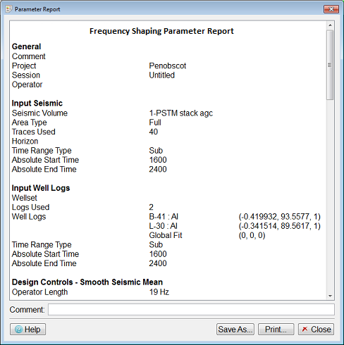
The figure above shows the "Parameter Report" dialog. This dialog displays the key parameters in the Frequency Shaping analysis and design phase nicely formated. Click the Save As... push button will pop up a file selector dialog allowing you to save to an ASCII file the formated parameter report.