To use this application to design the operators, it is first necessary to analyse the seismic and well data spectra. This is achieved by loading some seismic trace data and well log impedance data in time. Pop up the "Select Input Data" dialog by either clicking the menu item under the menu bar or by clicking the  icon.
icon.
The table below shows both tabs of the Select Input Data dialog with an example of data selected for the operators design. This application is data driven which means that the complete analysis and design of the operators (or as far as possible) are performed as soon as the data is loaded or updated.
This section describes how to select the input seismic trace data for use in the operators design. Frequency Shaping requires that you select a predetermined number of seismic traces from the full 3D survey area or sub-area, determined by the user. Trace selection is random within the area. Our aim is to select a set of traces which is representive of the 3D Survey Area for which we are trying to derive the operators. With the data selected it will normally be necessary to constrain it in some manner. The sub-section below describe how you can select and constrain the trace data.
This section allow you do specify the 3D Survey Area to be used to retrieve trace data for analysis.
| Input Seismic tab from the Select Input Data dialog | ||
|---|---|---|
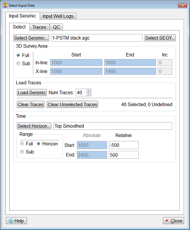 | The picture to the left shows the Input Seismic tab when using this tool as a plugin to OpendTect*. Seismic data can be selected by pressing the button. The seismic data selector will display all the available seismic cubes. If the volume list is long, then you can use the volume filter field to immediately reduce the number of entries thus making it easier to select the particular seismic volume needed for the analysis. * OpendTect is a trade mark of dGB Earth Sciences. ARK CLS aknowledges all third party trade marks. | |
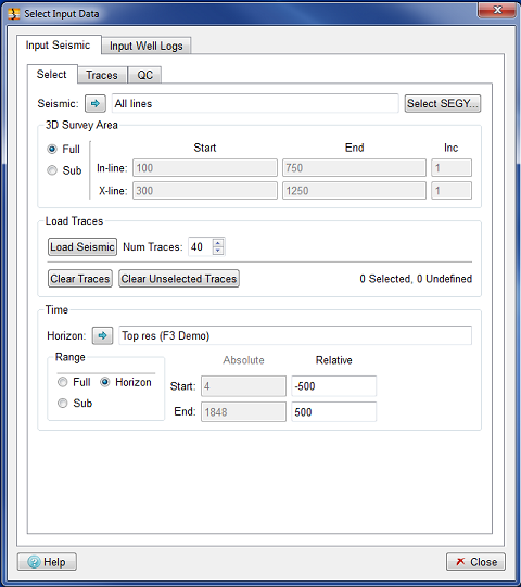 | The picture to the left shows the Input Seismic tab when using this tool as a plugin to Petrel*. The Seismic : Subsequent pictures in this section are of the OpendTect variant. * Petrel is a trade mark of Schlumberger. | |
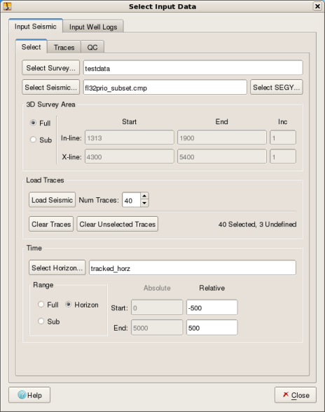 | The picture to the left shows the Input Seismic tab when connecting this tool to OpenWorks. Begin on this tab by selecting a Survey by pressing the button. After a survey has been selected seismic data can be selected by pressing the button. The seismic data selector will display all the available seismic cubes. If the volume list is long, then you can use the volume filter field to immediately reduce the number of entries thus making it easier to select the particular seismic volume needed for the analysis. In order to connect Frequency Shaping to an OpenWorks database it must be run within an OpenWorks environment. An OpenWorks System Terminal Window will provide a suitable environment. A Project must first have been selected from the Main Window's File -> DB Project selector. Subsequent pictures in this section are of the OpendTect variant. * OpenWorks is a trade mark of Halliburton. |
With the seismic data selected it usually desirable to define a sub-area. This is achieved by clicking the Sub button from the 3D Survey Area radio button group. Following this the user would select sub-area using the Start In-line, End In-line, Start X-line and End X-line edit boxes. Finally, the number of traces is specified and the button is clicked.
With the seismic data volume selected you can now load a set of traces to be analysed. Here you can optionally choose to select traces from the full 3D survey area or sub 3D survey area. This is achieved using the radio button group as follows:
for the complete area
and setting the In-line and X-line Start and End values for a sub-area
Typically you would select a single sub-area. Specifying a sub-area in this manner enables you to include an area of the survey where the trace data is known to be of good quality and isrepresentative of the survey area as a whole. With sub-area selected it is simpliy a case of specifying the number of traces to load (default 40) via the Num. Traces input field widget. This is then followed by you clicking the button to load a random set of traces. A list of the randomly loaded traces is then displayed beneath the button.
This software also enables to select trace data from multiple sub-areas. This is achieved by specifying another In-line/X-line Start and End range and clicking the button again. The goal is to generate seismic trace spectral which is good representation of the area as a whole. If you attempt to specify an area which is outside of the available area then a warning message will be issued when you attemp to load seismic traces by clicking the button.
You will also get an error message if you set an area which would not allow enough unique traces for the Num. Traces requested.
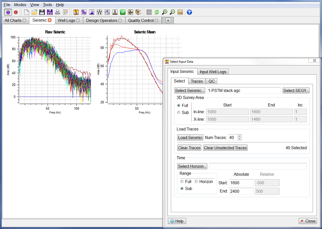 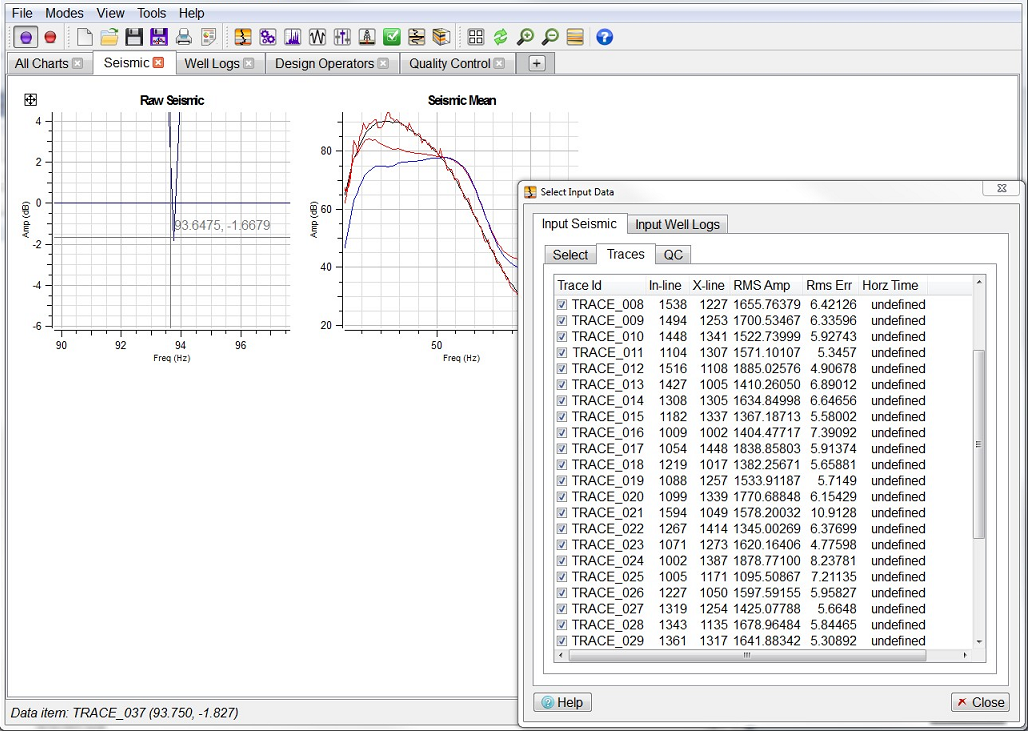 | The Main Window with Select Input Data Dialog superimposed (top left) shows the Raw Seismic spectra resulting from clicking the button on the "Select Input Data Dialog" (above left) with Num. Traces set to 40 and a 3D Survey Area defined by: In-line: 1000 - 1600 X-line: 1000 - 1480 By default, all loaded traces are used in the spectra calculation and contribute to the Seismic Mean Spectrum. If one or more seismic trace spectra displayed on the Raw Seismic plot were anomalous then it is possible to remove those traces from the Seismic Mean Spectrum calculation. Let us imagine our Raw Seismic chart shows there is a trace with anomalous amplitudes that are biasing the mean. Now if we wish to exclude this trace from the mean calculation, we must first identify it. This is achieved by pointing at one of the vertices of this spectrum and click on it. We need to be within one pixel of the vertices to be able to identify it, being anywhere on the plotted line is not sufficient. If we are within range when we click then the spectra name together with the Frequency and Amplitude of the vertice is displayed in the Status Area of the Main Window. Suppose the raw seismic spectra is identified as "TRACE_036". We can now to go to the Input Trace list and click checkbox to the left of entry "TRACE_036. This causes the trace to be flagged as not currently selected and the Raw Seismic plot on the Main Window is updated accordingly. The Seismic Mean spectrum (black) on both displays changes as a consequence. |
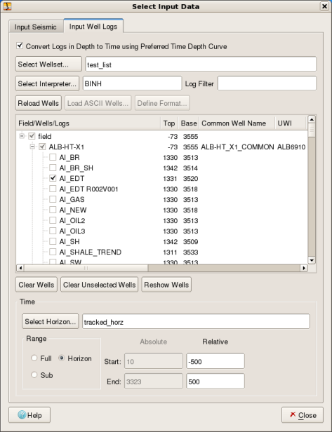
With the "Select Input Data" dialog displayed click the "Input Well Log" tab to select the well log data to use. This software supports reading acoustic impedance in time, from ASCII files or by connection to OpendTect. Here we shall assume you will normally wish to obtain data from OpendTect well log data repository and we will describe this route. If you wish to load from ASCII files then please refer to the full User Manual.
| Input Well tab from the Select Input Data dialog | ||
|---|---|---|
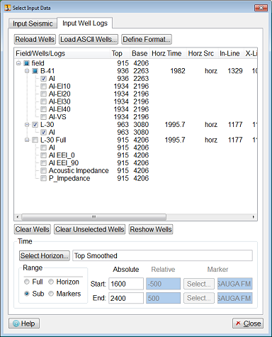 | The picture to the left shows the Input Well Logs tab when using this tool as a plugin to OpendTect. Clicking the push button will auto select acoustic impedance log curves in the OpendTect data repository. It is assumed that acoustic impedance log will have the characters "AI" (upper or lower case) or "IMP" (upper or lower case) somewhere within the log curve name. If, for a given well, there are no such acoustic impedance log curves or the log curve doesn't meet the assumed naming convention, then the user can still select or generate AI log curves manually. This is achieved by right clicking on the well name after first attempting to load the wells automatically. Note the push button will change to a push button after the initial automatic selection. Right clicking will pop-up a menu with and menu items. Selecting the first item will pop-up the "Select Database Logs" dialog which lists the available logs allowing you to choose an AI log curve however it is named. Selecting the second item will pop-up the "Generate AI Log" dialog which displays two lists. The left hand list allows you to select a sonic log and the right hand list allows you to optionally select a density log. If no density is available, then you can select for Density Source radio button and for supplying a User Density Value. Here the AI log will be generated from the supplied sonic and density. In OpendTect log curves are stored in depth, while this software requires the AI log curves to be in time. This transformation and resampling is done automatically, using the Depth/Time model allocated for each well. This data in the time domain can be displayed on one or more Main Window charts. By default, the AI data (in time) is displayed on the "Log Input (time domain)" and "Log Input Detrend (time domain)" charts. As each AI log curve is loaded its amplitude spectra are also immediately calculated and displayed by default on the "Individual Wells" chart. | |
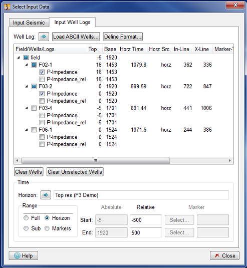 | The picture to the left shows the Input Well Logs tab when using this tool as a plugin to Petrel*. Select a well folder or individual well log in the Petrel input treee then click the Well Log: Single log: If a single continuous log is currently selected in the Petrel input tree, it will be shown in the input well logs "Field/Wells/Logs" table and will be selected by default. Multiple logs: If multiple logs are currently selected within the Petrel input tree, those representing continuous logs will appear in the table, but will not be selected by default. Wells: If wells or well folders are selected in the Petrel input tree, they will be searched, and all continuous logs with units suitable for Acoustic Impedance will be loaded into the "Fields/Wells/Logs" table. | |
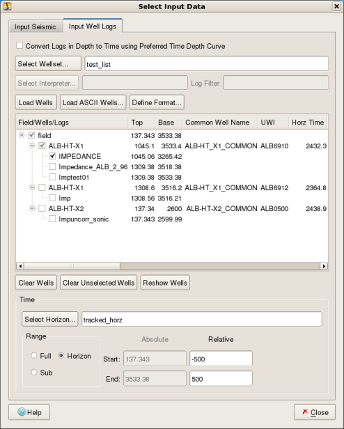 | The OpenWorks Input Well Logs window when using synthetic seismic AI logs in time. The image in the figure above shows the Input Well Log tab, used to load OpenWorks well log AI data. The image shows the check box is un-checked meaning that AI logs in time stored as synthetic seismic will be read from the database. Click the push button to pop up "Select Wellset" dialog (see Section Wellset dialog below). If no well data has been previously selected then clicking the will also pop up the "Select Wellset" dialog. From the "Select Wellset" dialog highlight the Wellset you require and click the push button. This will cause all AI data logs which have the specified naming convention to be automatically loaded but not selected for the OpenWorks Wellset. You can then select from the list the AI data logs you wish to use in the analysis. It is assumed that acoustic impedance logs will have the characters "Imp" (upper or lower case) somewhere within the log curve name or "Impedance" (upper or lower case) in the remark field. If, for a given well, there are no such AI log curves or the log curve doesn't meet the assumed naming convention, then the you can still load AI log curves manually. The image shows, in the central area, that three AI log curves, two for the ALB-HT-X1 well and one for the ALB-HT-X2 well, have been automatically loaded. Here we have selected one AI curve from just one well. We can also manually select AI well logs. This is achieved by right clicking on the well name which will pop-up a menu with Selecting this item will pop-up the "Select Database Logs" dialog which lists the available logs allowing you to choose an AI log curve however it is named. | |
 | The OpenWorks Input Well Logs window when converting depth logs to time. The image at left show the alternate OpenWorks situation where AI logs are loaded from depth logs which are automatically converted to time using the interpreter's preferred time depth curve. The check-box is checked which enables the selection of an interpreter using the push-button. After the selection of the Wellset (see above in the Synthetic Seismic case) a window pops up that displays a list of interpreters for the project. Following the selection of the Interpreter the list will be populated with logs that have been converted from depth to time using the Interpreter's preferred time depth curve. If no logs are converted for a particular well a warning will be displayed. |
The list below show the steps to generate well log spectra:
Load Wells
Details of loading wells for each of the variants are described above.
General to every variant, the central area of the Input Well Log tab shows the available AI log curves for each well. You can deselect wells and/or log curves by clicking on the appropriate .
Set Time Range
Again our aim is to design operators for the zone of interest (target). It is therefore desirable to time gate the selected traces prior to generating well log spectra. Ideally you should use a well defined interpreted horizon in the target zone to guide the well log trace time gate. In this manner the various gated log traces should have sample values over a similar geology.
Click to pop up a horizon select dialog, select the horizon you require and then click button to return.
Click in the Range radio button and specify the Relative Start and Relative End values. A negative number is a relative time above the horizon (i.e. shallower) and a positive number is a relative time below the horizon (i.e. deeper). The aim is to select a time gate which has a gate length within the range 500 - 1000 msec. The user supplied values here are accepted, and the chart area updates when you do any of the following: press Return key, press Enter key, press Tab key or mouse click on a different widget.
Apart from the horizon time gating you can also time gate your well data by using absolute time values with the Full and Sub options, but also by using markers*. When time gating by using the markers option you must select two common markers between all the selected well logs to be used as start and end times. The Relative Start and Relative End values are now relative to the start and end markers. Note that the same marker can be chosen for both the start and end. *Note that markers are not available in the OpenWorks connected variant.
With the seismic and well data loaded, the application will complete all the various steps to generate both Low End and High End operators. However, with this data driven approach the initial derived operators may not be optimum. As such, it may be necessary for you to perturb some of the design parameters before saving the operator. Apart from controlling desired data and data ranges, all other design parameters are accessible via the Design Operator and the Advanced Controls dialogs.