This section describes how to select the input seismic trace data for use in the Spectral Blueing operator design. Spectral Blueing requires that you select a predetermined number of seismic traces from the full 3D survey area or sub-area, determined by the user. Trace is random within the area. Our aim is to select a set of traces which is representative of the 3D Survey Area for which we are trying to derive a Spectral Blueing operator. With the data selected it will normally be necessary to constrain it in some manner. The sub-section below describes how you can select and constrain the trace data.
This section provides a push button which will allow you to pop up a seismic selector dialog. The type of seismic selector will depend on whether the database you are connecting with is either a 3D project, a 2D project or SEGY file in Database Project mode. In File Project mode it will only be possible to select from a SEGY file . The Selector dialog displayed will configure itself automatically when clicking the push button. Note: these images were generated when SsbQt was run in an OpenWorks R5000 environment.
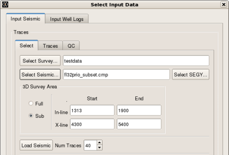
The figure above shows the top portion of the Input Seismic tab where a 3D seismic data volume has been selected. This is the standard way of selecting 3D seismic data volume when using the software with Landmark's SeisWorks or Schlumberger's GeoFrame data repositories.
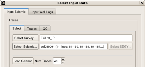
The figure above shows the top portion of the Input Seismic tab where 2D seismic lines have been selected.
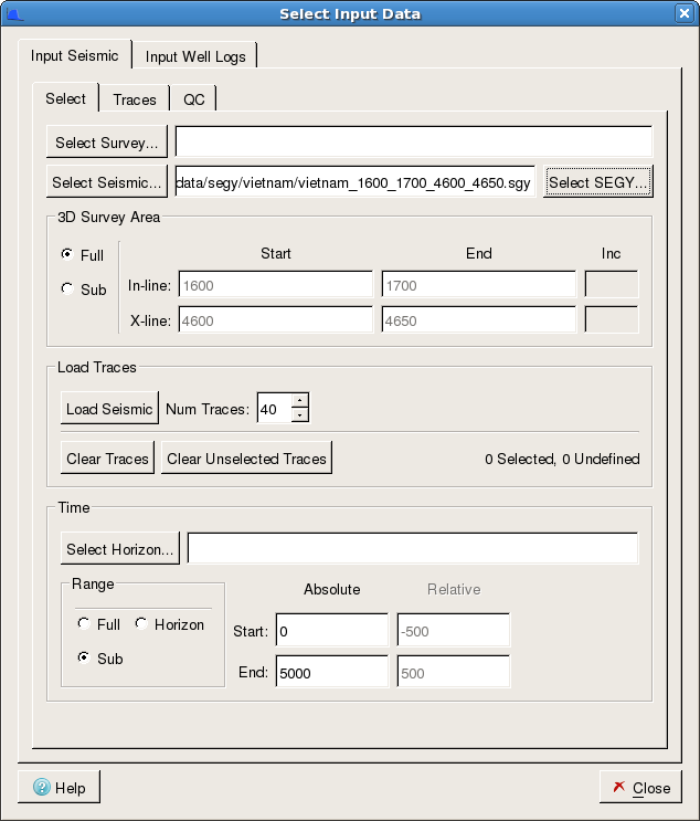
The figure above shows the top portion of the Input Seismic tab where a 3D SEGY file has been selected. Note the absence of the push button indicating that the software is in File Project mode.
With the seismic data volume selected you can now load a set of traces to be analysed. Here you can optionally choose to select traces from the full 3D survey area or sub 3D survey area. This is achieved using the radio button group as follows:
for the complete area
for setting the In-line and X-line Start and End values for a sub-area
Typically you would select a single sub-area. Specifying a sub-area in this manner enables you to include an area of the survey where the trace data is known to be of good quality and is representative of the survey area as a whole. With sub-area selected it is simply a case of specifying the number of traces to load (default 40) via the Num. Traces spinbox widget. This is then followed by you clicking the button to load a random set of traces. A list of the randomly loaded traces is then displayed in the Input tab beneath the button. At the same time an alternative set of traces is also loaded. These alternative traces are listed in the QC tab and are used with the derived Spectral Blueing operator for QC purposes. The software also enables you to select trace data from multiple sub-areas. This is achieved by specifying another In-line/X-line Start and End range and clicking the button again. The goal is to generate seismic trace spectra which is a good representation of the area as a whole. If you attempt to specify an area which is outside of the available area then a warning message will be issued when you attempt to load seismic traces by clicking the button. You will also get an error message if you set an area which would not allow enough unique traces for the Num. Traces requested.
Note: the following image illustrates the Landmark R5000 version of the Select input Data dialog which includes a button and text area.
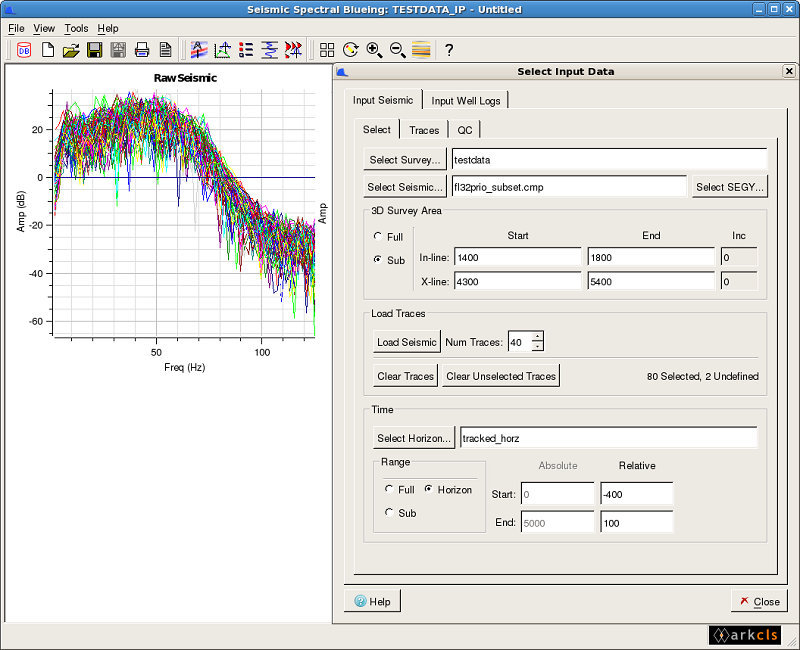
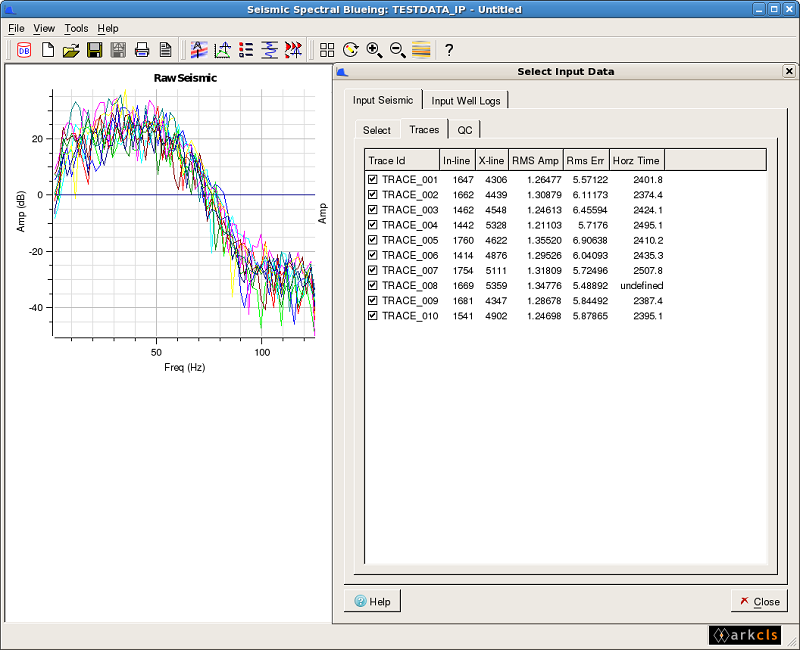
The image in the figure above shows the SsbQt Main Window with Select Input Data Dialog superimposed. The Raw Seismic spectra resulting from clicking the button on the "Select Input Data Dialog" (above left) with Num. Traces set to 40 and a 3D Survey Area is defined by:
In-line: 1400 - 1800
X-line: 4300 - 5400
By default, all loaded traces are used in the spectra calculation and contribute to the Seismic Mean Spectrum. However, you can remove a given trace from the SsbQt analysis by deselecting it via the Input list. Deselection of a trace is simply achieved by unchecking the checkbox within the list. If you want to completely remove the deselected trace you click the button. Alongside each trace on the Input list, are various properties associated with the trace. These include Trace Id (or trace label), In-line, X-line, RMS Amp, RMS Err, Horz Time. The RMS Amp property is derived from the input seismic trace, whereas the RMS Err property is derived from the trace spectrum. The latter can be considered as a "goodness of fit" parameter as it compares trace spectrum with the smooth mean trace spectrum. So for RMS Err, the smaller the number the better the fit. Loaded traces, by default, are sorted by Trace Id. However, you can sort the list of traces using one of the other properties. This is easily achieved by clicking the column header on the Input list. So, for example, if you want to sort by RMS Amp in ascending order, you click the RMS Amp header label. To sort in descending order you click the RMS Amp header label again. You can also change the position of the property columns. This is simply achieved by clicking and holding on a property header then dragging the property header to its new position.
The image shows the result of clicking the push button. Here 40 traces have been randomly loaded and immediately displayed in the "Raw Seismic" chart within the SsbQt Main Window. Also visible is a portion of the "Select Input Data Dialog" showing the trace list on the "Input" tab sorted by ascending RMS Amplitude values.
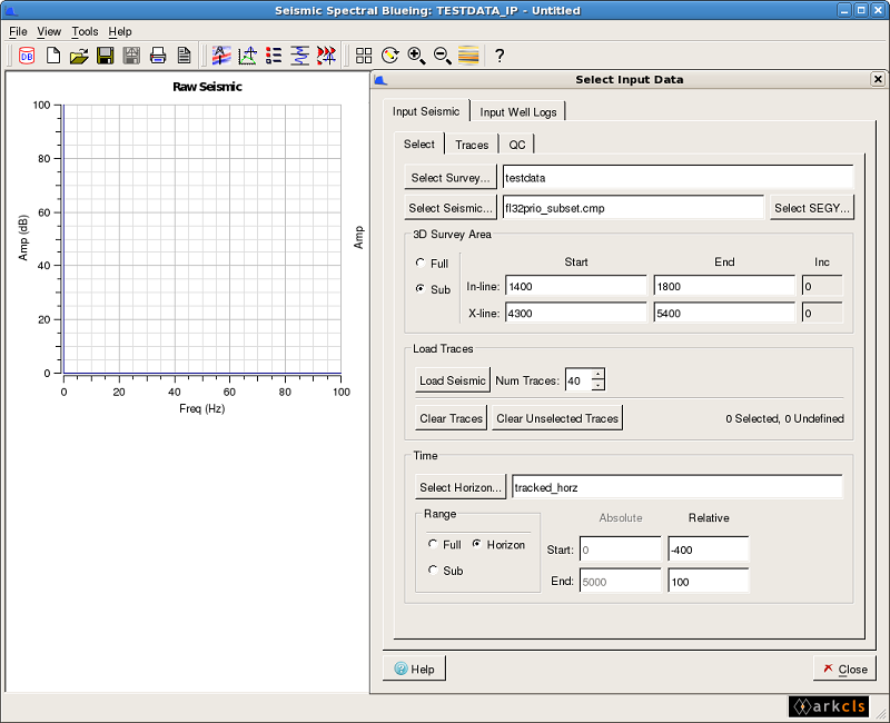
The image in the figure above shows the result of clicking the push button. Clear traces removes all traces previously loaded to memory and has the immediate effect of removing this data from the "Raw Seismic" chart within the SsbQt Main Window.
Specifying the time range (gate) is an important step. Ideally, you should choose a time gate in the range of 500 - 1000 msec which should be over the zone of interest. You can set the Time Range mode in one of three ways via the "Range" radio button.
Full - this range would cover the full trace length. It is rarely used
Sub - here you additionally need to specify Absolute Start Time and Absolute End Time. This Time Range mode is the default.
Horizon - here you additionally need to specify the Relative Start Time and Relative End Time. You also need to specify the horizon to be used.
Of the three options the Horizon Range mode is the preferred mode since it allows the gate to follow the geology and should, with a well interpreted horizon in the target zone give, in theory, trace spectra which are more closely matched.
Note: the following image illustrates the Landmark R5000 version of the Select input Data dialog which includes a button and text area.
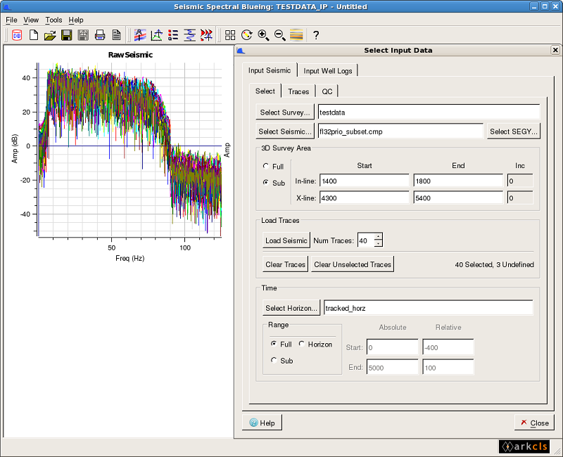
The image in the figure above shows the SsbQt Main Window with Select Input Data Dialog superimposed. Here, "Full" (full trace range) has been selected for the radio button. This mode is rarely used since our goal is to design a Spectral Blueing operator over the zone of interest. This will optimise the process over that zone. However, it does allow you, although insensitive, to see the start and end times of the entire trace.
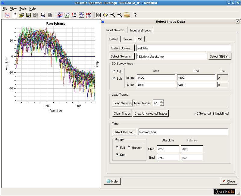
The image in the figure above shows the SsbQt Main Window with Select Input Data Dialog superimposed. Here, "Sub" (sub trace range) has been selected for the radio button. In this mode the Absolute Start time and the Absolute End time Line Edit fields will be sensitised. This allows you to specify a time gate for the zone of interest. Typically, you would specify a time gate which has a time range between 500msec and 1000msec.
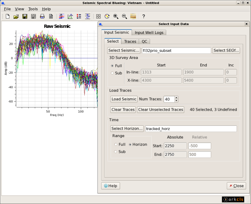
The image in the figure above shows the SsbQt Main Window with Select Input Data Dialog superimposed. Here, "Horizon" (horizon relative trace range) has been selected for the radio button. In this mode the Relative Start time and the Relative End time Line Edit fields will be sensitised. This allows you to specify a time gate for the zone of interest. Typically you would specify a time gate which would give you a time range between 500msec and 1000msec. Specifying the Start and End times here are relative to a geologic horizon. A negative number represents time above the horizon whereas a positive number is a time below the horizon. The time gate can be either above, below or span the horizon.
Occasionally, it is necessary to remove one or more poor spectral traces which contribute to the generation of the mean spectra. This is easily achieved by identifying problem spectral traces from the chart and deselecting these traces from within the Select Input Data Dialog.
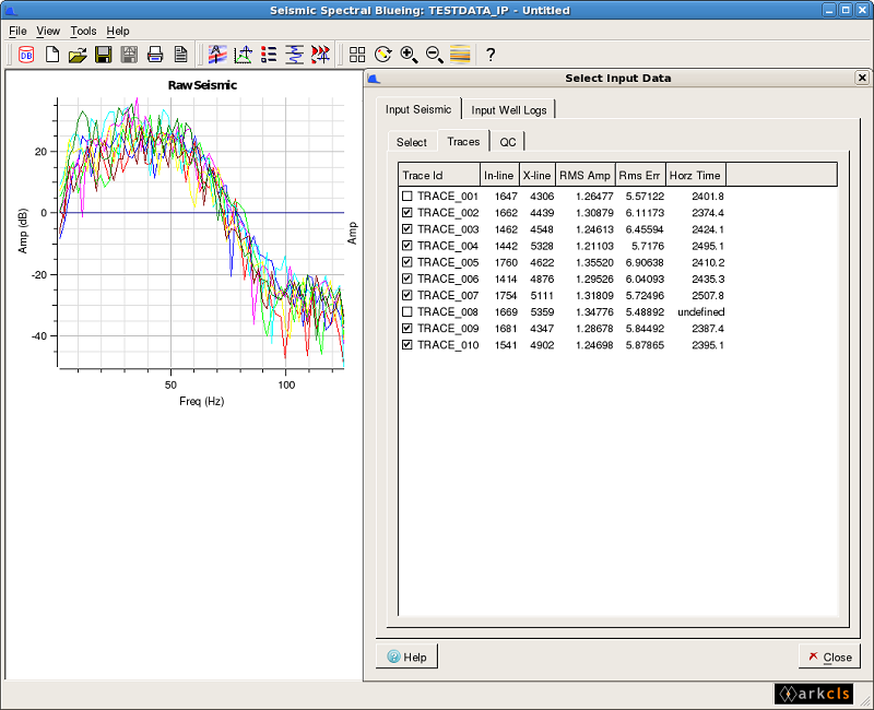
If one or more seismic trace spectra displayed on the Raw Seismic plot were anomalous then it is possible to remove those traces from the Seismic Mean Spectrum calculation.
To exclude a trace from the mean calculation it must first be identifed. This is achieved by pointing close to one of the vertexes of this spectrum and clicking on it. This should be within few a pixels of one of vertexes. If within range then the required spectra name together with the Frequency and Amplitude of the vertex is displayed in the Status Area of the Main Window. Having obtained the name go to the Input Trace list and uncheck the checkbox left of the required trace. This causes the trace to be removed and the Raw Seismic plot on the Main Window is updated accordingly. The Seismic Mean spectrum (black) on both displays also update. Alternatively examine the RMS Err property values and exclude traces that have significantly higher values than the other trace spectra. Sorting by RMS Err simplifies the task. Note that once a trace is toggled off the RMS Err is not calulated.
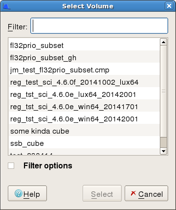
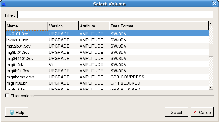
The Select Volume dialog provides you with a 3D seismic volume selector. From here simply select the seismic volume you require for your SsbQt analysis and operator design. A volume filter is provided to reduce the list to a manageable size for projects with many volumes.
 ...
...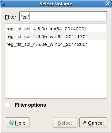
The images in the figure above show examples of the "Select Volume" dialog for selection of a seismic volume. The LH image shows a seismic volume list without a seismic volume filter. The RH image shows the use of a filter to create a shorter list. As can be seen, the wild card character (*) can be used in the Filter field.
The Select Volume dialog provides you with a 3D seismic volume selector. From here simply select the seismic volume you require for your SsbQt analysis and operator design. With OpenWorks R5000 volumes are identified by two data keys, Name and Version. Two additional attributes, Attribute and Data Format have been included for information. A Filter is provided to reduce the list to a manageable size for projects with many volumes. The column to filter can be controlled by the Filter Column menu. In the RH image the list has been filtered to include only those volumes which have V1 in the Version.
 ...
...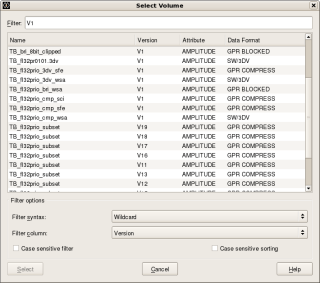
The images in the figure above show examples of the "Select Volume" dialog for selection of a seismic volume. The LH image shows a seismic volume list without a seismic volume filter. The RH image shows the use of a filter to create a shorter list. As can be seen, the wild card character (*) can be used in the Filter field.
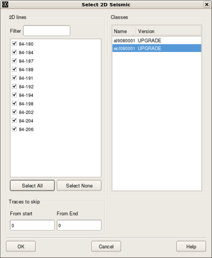
The Select 2D Seismic dialog provides you with a 2D seismic line selector. From here you select the 2D lines you require for your SsbQt analysis and operator design. A 2D line filter is provided to reduce the list to a manageable size for projects with many 2D seismic lines. Note: the images below show dialogs from the the R5000 version which has Name and Version to define the Classes.
 ...
...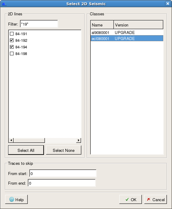
The images in the figure above show examples of the "Select 2D Seismic" dialog for selection of 2D seismic lines. The LH image shows seismic lines listed without a 2D line filter. The RH image shows the use of a filter to create a shorter list. As can be seen, the wild card character (*) can be used in the Filter field. From the list of available 2D lines (optionally filtered) you can select one 2D line to be included by clicking the unchecked check box to the left of a 2D line name. Multiple 2D lines can be selected by repeating this step. All 2D lines can be selected by clicking the push button. De-selection of a single 2D line is achieved by clicking a checked check box to the left of a 2D line name. All 2D lines can be de-selected by clicking the push button. With the 2D lines selected you must then select a class. Optionally you can skip traces at the start and end of each 2D line. This is achieved by specifying the Traces to skip via the From Start and From End line edit fields.
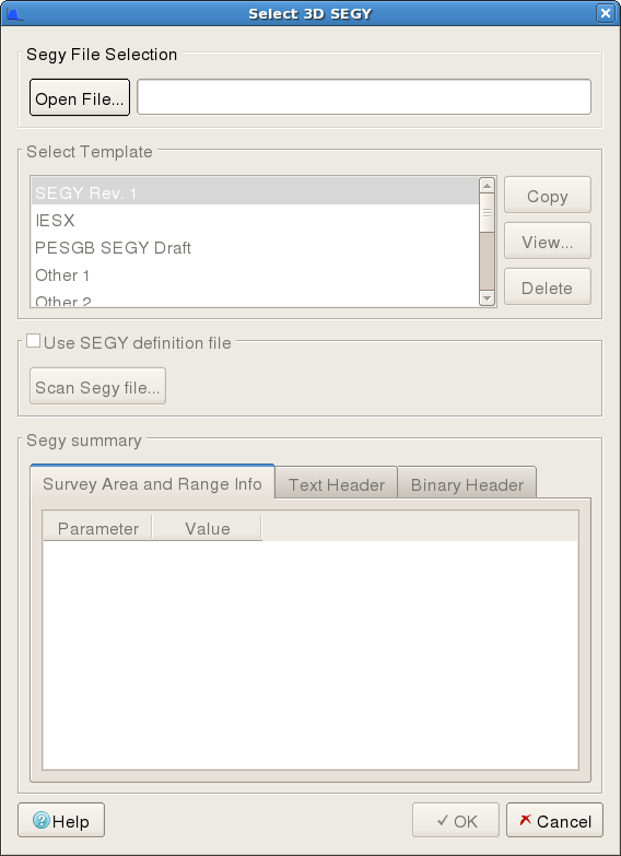
The Select SEGY dialog provides you with a 3D SEGY file selector. From here you select the 3D SEGY file you require for your SsbQt analysis and operator design. Unfortunately, selecting a 3D SEGY file for input here is not the end of the story. You need to also either select or build an offset mapping template for use with the selected SEGY file. Fortunately, within the software this is a straightforward task.
 ...
...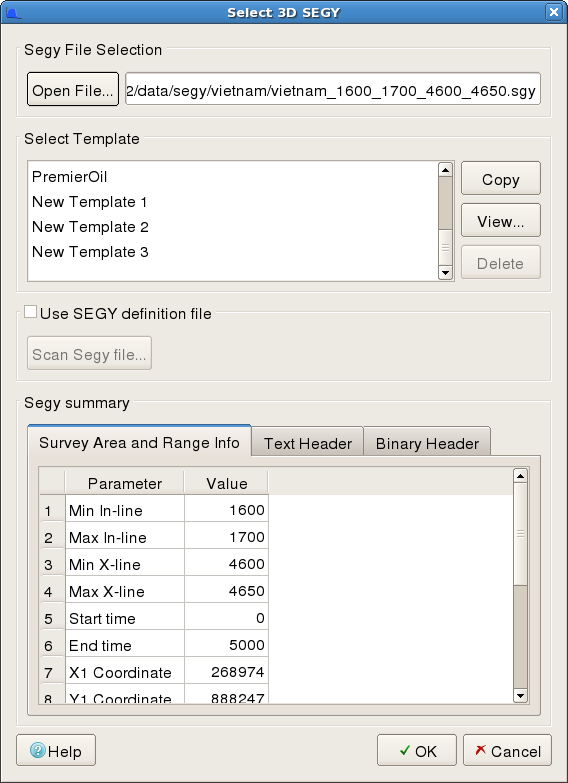
The images in the figure above show examples of the "Select SEGY" dialog for selection of SEGY files and offset mapping. The LH image shows the dialog prior to opening a SEGY file. To open a SEGY file click the push button which will pop-up a file selector dialog allowing you to traverse the file system to select and open a SEGY file. The RH image shows that a SEGY file has been opened and has been matched with an offset Template. In this case, it was matched with the "Other 1" template. This dialog attempts to automatically match the opened SEGY file with one of the available templates. If the match is successful then the matched template will be highlighted and Min/Max Inline/Xline together with Start/End Time obtained from the Opened SEGY file will be displayed in the "Survey Area and Range Info" tab within the "Segy Summary" block. Similarly the opened SEGY file's EBCDIC header information will be displayed in the "Text Header" tab with the SEGY Binary header information being displayed in the "Binary Header" tab.
Now, if no template match is found then it will be necessary to create a new template. Fortunately, this is a relatively simple process and is achieved in the following manner. Select an existing template, it doesn't really matter which one you use, then click the push button. Now select the new template which will appear at the end of the list of templates and will have a default name similar to "New Template 1". Finally click push button to pop up "Edit Template" dialog.
The Edit Template dialog provides you with a mechanism to edit SEGY templates. The original SEGY standard (rev 0) has been used extensively within the oil and gas industry as a convenient way to exchange seismic data between various companies. This standard was published in 1975 for storage of 2D line seismic data on magnetic tapes. Since this original publication there have been many advancements in geophysical data acquisition including disc recording and 3D seismic. The SEGY standard was subsequently used in ways that were never originally envisioned. Inevitably, this led to inconsistent use of the trace header attributes by different companies for storage of 3D seismic on disc. Whilst the SEGY standard (rev 1) published in 2002 was designed to address such issues, there is still a need to map (set up offsets) various trace header attributes as there is software and old SEGY files in existence that don't adhere to the new SEGY rev 1 standard.
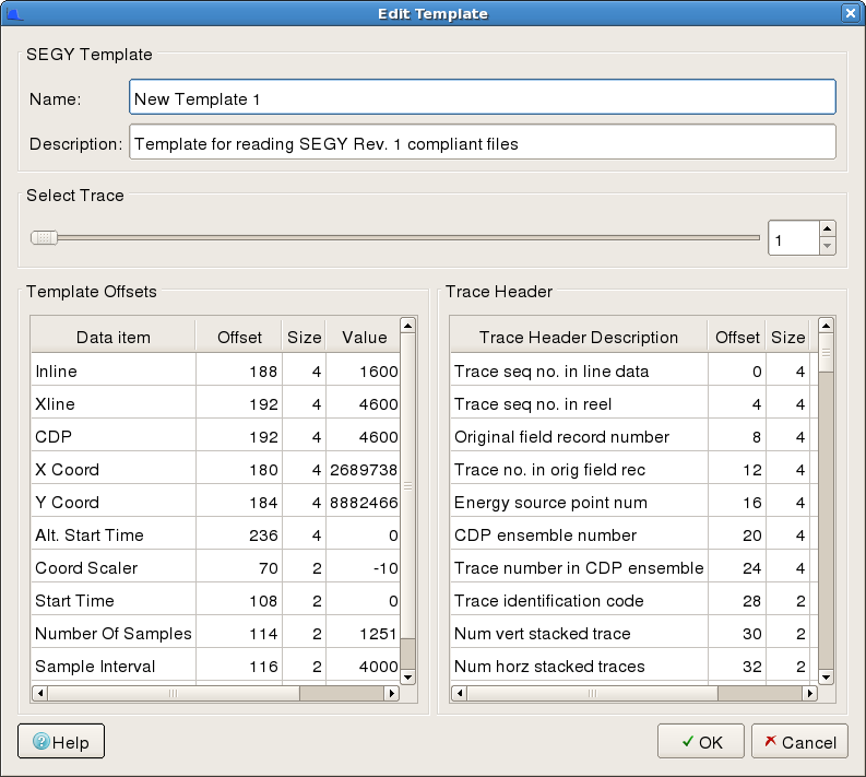
The figure above shows the "Edit Template" dialog. This dialog allows you to assign a unique name and add a brief description. The main purpose of this editor is to allow you to set up the Template Offsets for mapping various trace attributes.
OK, let's look at how we set up the various Template Offsets. This dialog works with the opened SEGY file. Within the "Select Trace" block there is a slider and a spin box object. Both allow you to move to different traces within the SEGY file. Using these objects you can position the trace reader to any trace within the SEGY file. So for any trace you will be able to display the trace header data in the right panel beneath "Trace Header" label. By scanning the trace header for a given SEGY trace you should be able to determine where in the header various pieces of information are stored. So to edit the template offset we do the following:
Determine for a given "Data item" where in the trace header this information is stored. In the above figure we look for inline in the trace header. In this case we find the Inline data is stored in trace header "Original field record number" which is at offset 8.
We grab this item (press and hold mouse button 1) and pull it to the LH side to the "Template Offset" we wish to set.
Once we are over "Template Offset" item we wish to update we let go the button on the mouse.
The "Template Offset Data item" will then show the same "Offset", "Size" and "Value" as in the trace header.
Steps 1-4 above are repeated for all "Template Offset Data items".
Whilst ARK CLS recommends that when creating a new Template all Data items are mapped, it may be possible to generate a Template without mapping every Data item in the Template Offset list. We consider the most important items are "Inline", "Xline", "X Coord", "Y Coord", "Coord Scaler", "Start Time", "Number Of Sample", "Sample Interval" and "Trace ID Code". These "Data Items" in the "Template Offsets" list should always be set.
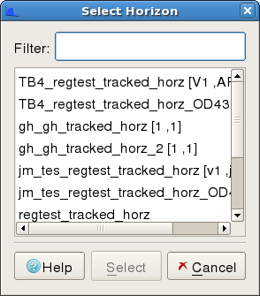
The Horizon Input Dialog provides you with a horizon selector. From the Horizon Data tab, simply select the horizon you require for your SsbQt analysis and operator design. A Horizon filter is provided to reduce the list to a manageable size for projects with many horizons.
 ...
...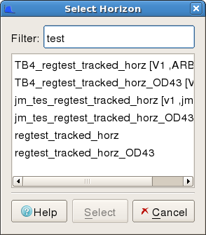
The images in the figure above show examples of the "Select Horizon" dialog for selection of a seismic horizon. The LH image shows a seismic horizon list without a horizon list filter. The RH image shows the use of a filter to create a shorter list. As can be seen, the wild card character (*) can be used in the Filter field.
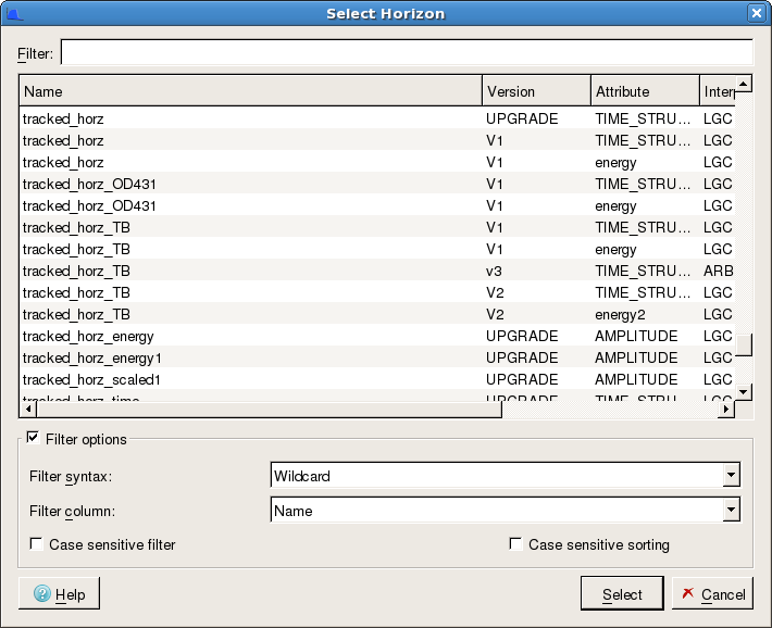
The Horizon Input Dialog provides you with a horizon selector. From the Horizon Data tab, simply select the horizon you require for your SsbQt analysis and operator design. With OpenWorks R5000 Horizons are identified by four data keys, Name, Version, Attribute and Interpreter. A Horizon Filter is provided to reduce the list to a manageable size for projects with many horizons.
 ...
...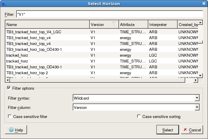
The images in the figure above show examples of the "Select Horizon" dialog for selection of a seismic horizon. The LH image shows a seismic horizon list without a horizon list filter. The RH image shows the use of a filter to create a shorter list. The column to filter can be controlled by the Filter Column menu. In the RH image the list has been filtered to include only those horizons which have V1 in the Version name.
When using a File Project (or running stand-alone on Windows) the database selector automatically switches to an ASCII horizon file selector. Firstly use the Open file... button to browse for the horizon file. When selected it is automatically read and the column data is displayed below. Set the values for Start reading at line:, In-line column:, Cross-line column: and Z data column: as appropriate. Press OK to load the horizon into the application.
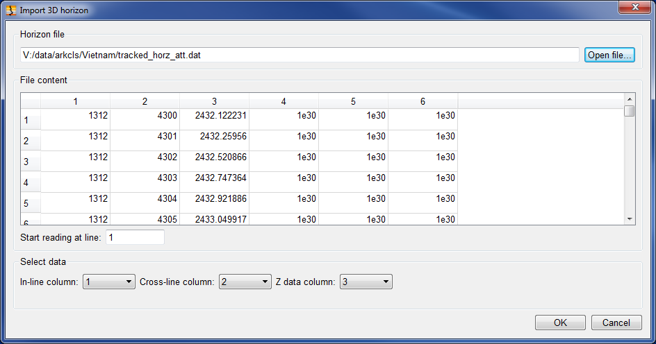
The figure above shows an example of the ASCII horizon selector with no header lines, inline values in column 1, cross-line values in column 2 and the Z values (Time) in column 3.
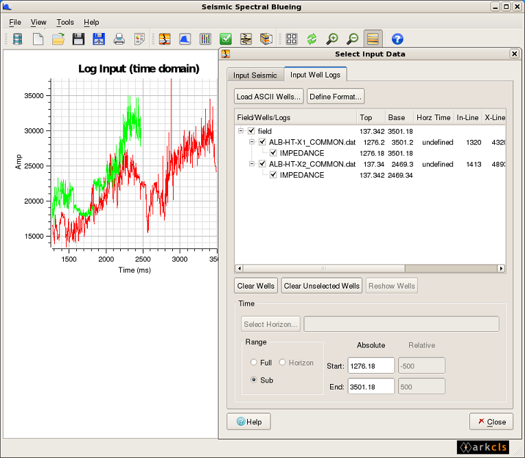
This section describes how to select the input well log Acoustic Impedance (Reflectivity) data for use in the Spectral Blueing operator design. Spectral Blueing requires that you select one or more Acoustic Impedance logs from those available for the project. These Accoustic Impedance logs are then used to generate Reflectivity. We use the reflection coefficient curves to generate spectra Ideally we would like to generate Reflectivity spectra from multiple well logs as this should help to retrieve a better global spectrum to curve fit. However, data from the different wells might be of variable quality so it is up to you to decide which wells to use. The figure below shows the Input Well Log tab on the Select Input Data Dialog.
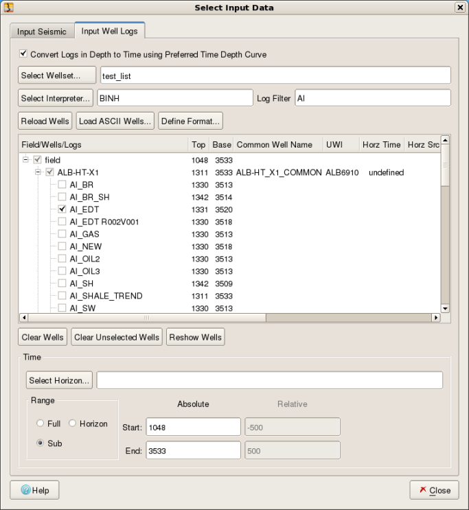
In the above dialog the large central area is to display and control the selection of Well Log Acoustic Impedance data. It can consist of the following fields: Field/Well/Logs, Top, Base, Common Well Nm, UWI, Remark, In-line, X-line, Horz Time and Horz Src. These fields can be moved by grabbing (click and hold) the field header and dragging to a new position. Clicking on the field headers sorts the list according to the data in that field. The Field/Wells/Logs provides a facility to expand and contract the entire list. Additionally, this field allows Acoustic Impedance data to be selected and deselected.
The sub-sections below describe how you can select and constrain the data.
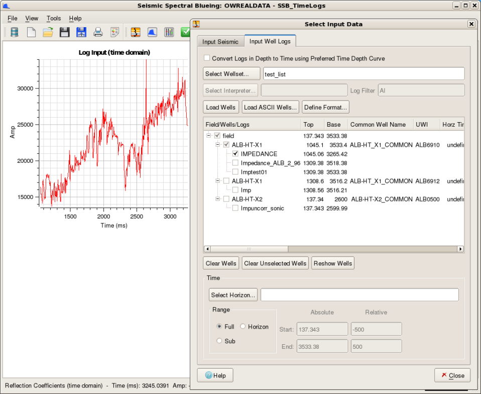
Loading acoustic impedance data from OpenWorks database is straightforward. GeoFrame database access is not currently supported in this release (see Load ASCII Wells...). Logs data, as used by SCI, is stored in the OpenWorks database as either synthetic seismic in time or as logs in depth. Acoustic Impedance logs stored as synthetic seismic traces in time are read and used directly. Logs in depth are converted internally to time using the interpreter's Preferred depth to time model for the selected wells. Details for loading Reflectivity data from OpenWorks are explained beneath.
 ....
....
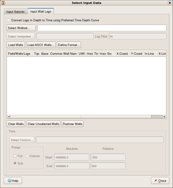
The two images in the figure above show the top portion of the Input Well Log tab, used to load OpenWorks well log Reflectivity data. The LH image shows the state when you pop up the "Select Input Data" dialog and click the "Input Well Logs" tab. Here the check box is un-checked meaning that Reflectivity logs in time stored as synthetic seismic will be read from the database. Click the push button to pop up "Select Wellset" dialog (see Section Wellset dialog below). If no well data has been previously selected then clicking the will also pop up the "Select Wellset" dialog.
From the "Select Wellset" dialog highlight the Wellset you require and click the push button. This will cause all Reflectivity data logs which have the specified naming convention to be automatically loaded but not selected for the OpenWorks Wellset. You can then select from the list the Reflectivity data logs you wish to use in the analysis.
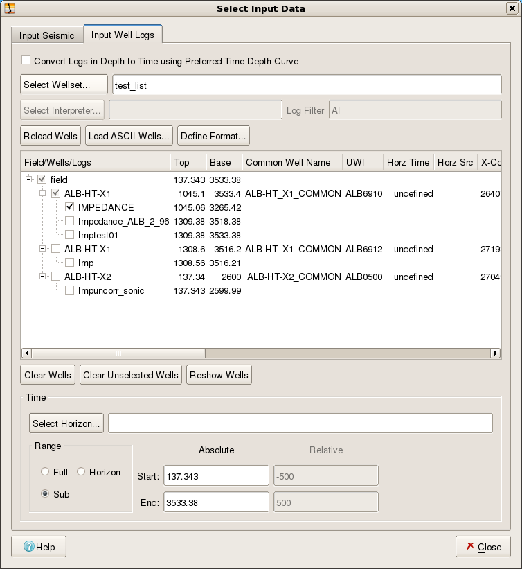
It is assumed that acoustic impedance logs will have the characters "Imp" (upper or lower case) somewhere within the log curve name or "Impedance" (upper or lower case) in the remark field. If, for a given well, there are no such Reflectivity log curves or the log curve doesn't meet the assumed naming convention, then the you can still load Reflectivity log curves manually.
The RH image above shows, in the central area, that three Reflectivity log curves, two for the ALB-HT-X1 well and one for the ALB-HT-X2 well, have been automatically loaded. Here we have selected one Reflectivity curve from just one well.
We can also manually select Reflectivity well logs. This is achieved by right clicking on the well name which will pop-up a menu with Selecting this item will pop-up the "Select Database Logs" dialog which lists the available logs allowing you to choose an Reflectivity log curve however it is named.
 ....
....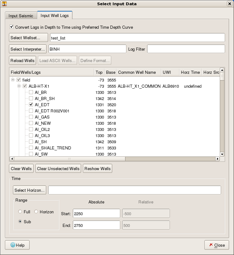
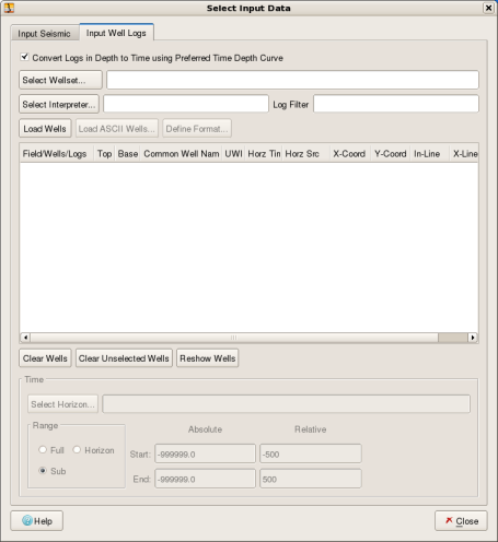
The two images above show the alternate situation where Reflectivity logs are loaded from depth logs which are automatically converted to time using the interpreter's preferred time depth curve. The check-box is checked which enables the selection of an interpreter using the push-button. After the selection of the Wellset (see above in the Synthetic Seismic case) a window pops up that displays a list of interpreters for the project. See section Select Interpreter dialog below.
A Log Filter field is provided to allow users to list only logs which match the filter. This defaults to "Reflectivity" but can be changed to any desired string EG "EI". If all the logs are required either a blank filter or "*" will list all the logs for each well. Note that listing all logs will considerably increase the time required to populate the list.
The push buttons and are self explanatory. The push button will re-display any of the wells/logs cleared via the and push buttons. Note the push button will change to a push button after the initial automatic selection. The push button will reload from the database all the currently available wells for the Wellset. In this way any new data loaded to the database will be displayed.
The Select Wellset dialog provides you with a well set selector. From here simply select the well set you require for your SsbQt analysis and operator design. A well set filter is provided to reduce the list to a manageable size for projects with many well sets.
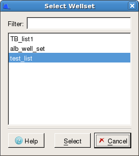
The image in the figure above show an example of the "Select Wellset" dialog for selection of an OpenWorks well set.
The Select Interpreter dialog provides you with a list of available interpreters for the project. This will be used to find the Preferred Time Depth Curve for each well in the wellset. Wells that do not have a Preferred Time Depth Curve for the selected interpreter cannot be time converted and therefore will be omitted from list of available wells. A warning message box pops up in this situation.
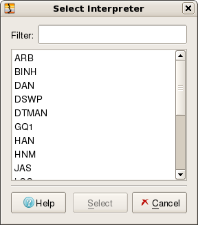
Example of a "Select Interpreter" dialog to select an OpenWorks interpreter.
The Select Database Logs dialog provides you with an Acoustic Impedance log selector. Here you can select any database log, in time, irrespective of how it is named. An acoustic impedance log filter is provided to reduce the list to a manageable size should there be many logs for the well.
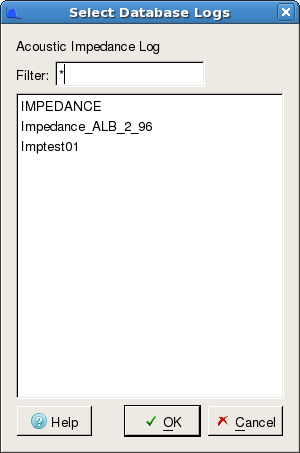
The image in the figure above shows an example of the "Select Database log" dialog for selection of OpenWorks impedance logs in time. Note only one Reflectivity log can be selected at a time. This window is reached by right-clicking on a well in the Field/Wells/Logs list.
Loading Acoustic Impedance data from ASCII is straightforward. Simply click on the push button to pop up a file selector. Within the File Selector you can traverse the file system to locate Acoustic Impedance data in ASCII format. The File Selector allows one or more ASCII files to be open at once. Use the <Shift> key modifier to select consecutive files and the <Ctrl> key modifier to select non-consecutive files from within the File Selector dialog. You can also MB1 and drag the mouse over a number of ASCII files.
The picture in the figure above shows the Input Well Log tab, where well log data has been loaded. In this case the well log data was loaded from ASCII files. The central list area shows four impedance curves have been loaded. One each for four wells. Normally, well log ASCII data files do not contain inline, xline or horizon data. So, in such cases, it is not possible to select a time range relative to an interpreted horizon. However, SsbQt recognises certain XML style meta tags, which can be used by you to provide additional data. Below are the five XML style meta tags recognised by SsbQt.
<inline>inline data here</inline>
<xline>xline data here</xline>
<horztime>horizon time data here</horztime>
<xcoord>x coordinate here</xcoord>
<ycoord>y coordinate here</ycoord>
These XML meta tags are normally inserted on one line within the ASCII file. For example, in Landmark style ASCII files these would normally be placed on the second line (which is blank). It is not necessary to include all the meta tags. Normally, only the <inline> and <xline> meta tags are supplied as there is then sufficient information for horizon data to be extracted from the supplied horizon. In this example, the horizon information for well_4.dat, well_3.dat and well_3.dat can be obtained from the supplied horizon (Horz Scr = horz) using the In-line and X-line data supplied via the meta tags <inline> and <xline>. For well_1.dat however, the horizon information comes from the <horztime> meta tag (Horz Scr = well) since no In-line or X-line data has been supplied.
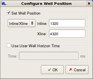
An alternate way to set the well position is interactively via a drop-down menu found by right-clicking on well name in the Field/Wells/Logs tree. Selecting will pop-up the window shown above. Enter the required in-line or cross-line location. Alternately the X/Y location can be entered instead. It is also posible to enter a well horizon time here if required.
This section describes how you can define the format for ASCII file reading of well Reflectivity log data. Clicking the push button will pop up the "Define ASCII File Format" dialog.
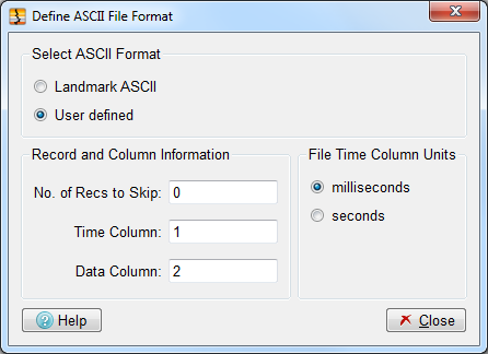
The figure above shows the "Define ASCII File Format" dialog. This dialog has three groups: "Select ASCII Format", "Record and Column Information" and "File Time Column Units".
Select ASCII Format: This group contains a radio button with two options and . In mode (default) the other two groups are desensitised. In mode you can supply additional information in the "Record and Column Information" and "File Time Column Units" groups. Although no explicit LAS input facility is provided, you can normally read LAS files in mode.
Record and Column Information: If your ASCII has header records before the wireline curve data you should skip these by specifying a value in the input field. You should also specify which column the time data and the log data can be found. By default, these are set to 1 and 2 respectively.
File Time Column Units: This radio button item allows you to specify whether the time data is in s or .
Specifying the time range (gate) is an important step. Ideally, you should choose a time gate in the range of 500 - 1000 msec which should be over the zone of interest. You can set the Time Range mode in one of three ways via the "Range" radio button.
Full - this range would cover the full trace length. It is rarely used.
Sub - here you additionally need to specify Absolute Start Time and Absolute End Time. This Time Range mode is the default.
Horizon - here you additionally need to specify the Relative Start Time and Relative End Time. You also need to specify the horizon to be used.
Of the three options the Horizon Range mode is the preferred mode since it allows the gate to follow the geology.
The image in the figure above shows the SsbQt Main Window with Select Input Data Dialog superimposed. Here, "Full" (full trace range) has been selected for the radio button. This mode is rarely used since our goal is to design a Spectral Blueing operator over the zone of interest. This will optimise the process over that zone. However, it does allow you, although insensitive, to see the start and end times of the entire trace.
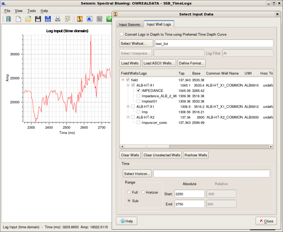
The image in the figure above shows the SsbQt Main Window with Select Input Data Dialog superimposed. Here, "Sub" (sub trace range) has been selected for the radio button. In this mode the Absolute Start time and the Absolute End time Line Edit fields will be sensitised. This allows you to specify a time gate for the zone of interest. Typically, you would specify a time gate which has a time range between 500msec and 1000msec.
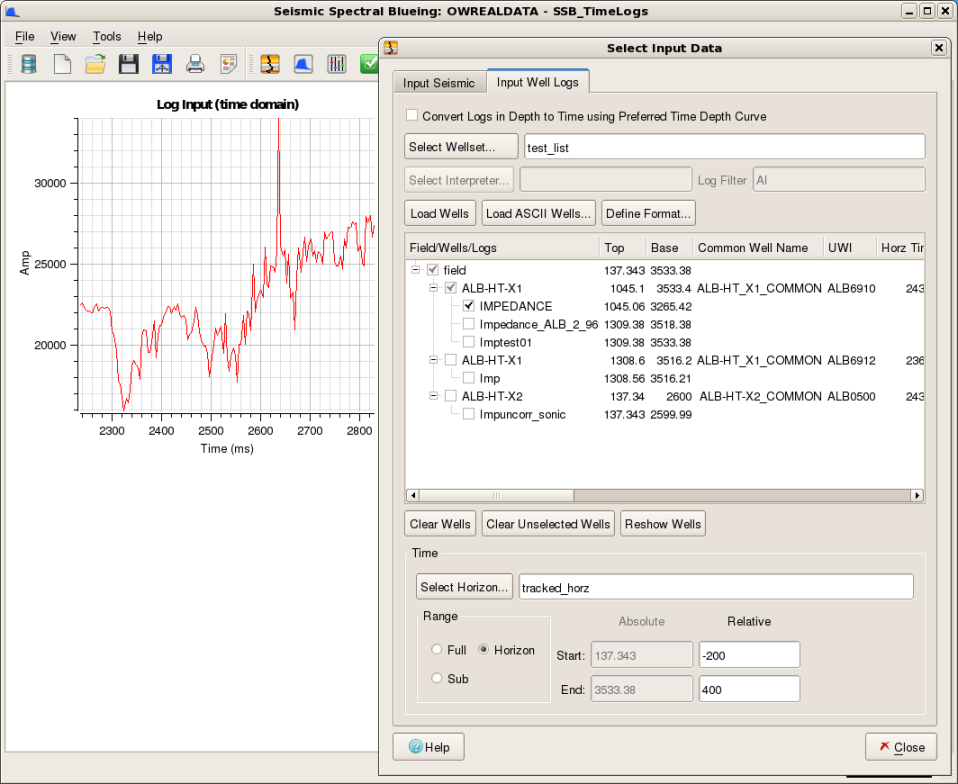
The image in the figure above shows the SsbQt Main Window with Select Input Data Dialog superimposed. Here, "Horizon" (horizon relative trace range) has been selected for the radio button. In this mode the Relative Start time and the Relative End time Line Edit fields will be sensitised. This allows you to specify a time gate for the zone of interest. Typically, you would specify a time gate which would give you a time range between 500msec and 1000msec. Specifying the Start and End times here are relative to a geologic horizon. A negative number represents time above the horizon whereas a positive number is a time below the horizon. The time gate can be either above, below or span the horizon. Clicking the push button will pop up the Horizon Input Dialog.