The input data tab is used to load and/or calculate the horizon attribute data and extents that will be used within the seismic net pay calculation. This tab is divided into two sub-tabs, Calculation and Load.
This section describes how to calculate the input 'Average Amplitude', 'Time Separation', and 'Gross Thickness' horizons used in the net pay calculation by providing a 'Coloured Inversion Volume', and top and base horizons for both time and depth.
To calculate the 'Average Amplitude' horizon attribute it is needed to have a 'Coloured Inversion Volume', a 'Top Time Horizon', and a 'Base Time Horizon'. These time horizons must be picked on zero crossings on Coloured Inversion data. If the reservoir is low impedance relative to non-pay then the top pick will be on a +/- crossing and the base pick will be a -/+ crossing. The reservoir interval should be isolated from other reflectors above and below it. The interval may contain multiple seismic loops but accuracy will decrease the thicker the interval. 'Average Amplitude' is then calculated by averaging the amplitude values of the 'Coloured Inversion Volume' between the 'Top Time Horizon' and the 'Base Time Horizon'. These values are then stored as an attribute on the 'Top Time Horizon'.
'Time Separation' is calculated between the top and base time horizon and 'Depth Thickness' is calculated between top and base depth horizons.
One, two or three output attributes will be calculated depending on the input data, as follows:-
If the user only selects the Top and Base Time Horizons, only the 'Average Amplitude' and 'Time Separation' can be calculated.
If the user only selects the Top and Base Depth Horizons, only the 'Depth Thickness' can be calculated.
If the user selects the Top and Base Horizons for both time and depth, then all the three input horizon attributes can be calculated.
NOTE: ASCII version users will need to set manually the horizons undefined value which will be required for both reading and writing of horizons.
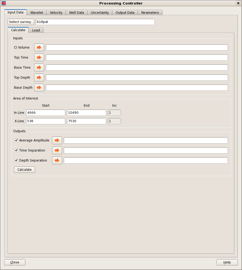
The following steps are taken in this tab before pressing the Calculate button:
Specify an area of interest, in terms of in-lines and cross-lines, for data loading and calculation.
Initially these values will be a calculated sub-set the AI Volume extents, but the user can edit the values to further sub-set the area of interest.
The Inline/Xline increment is not editable by default and is for information purposes only. However, if the input horizons are decimated, with for example, in-line and cross-line increments of 2, then it is possible to make the Inline/Xline increment editable by ticking on the the Parameters tab the Inline/Xline increment Allow override box. On returning to the Input Data tab the increments will be found to be editable.
After pressing the calculate button, the horizon attributes are then calculated and automatically loaded.
This section describes how to load the input 'Average Amplitude', 'Time Separation', and 'Gross Thickness' horizons used in the net pay calculation.
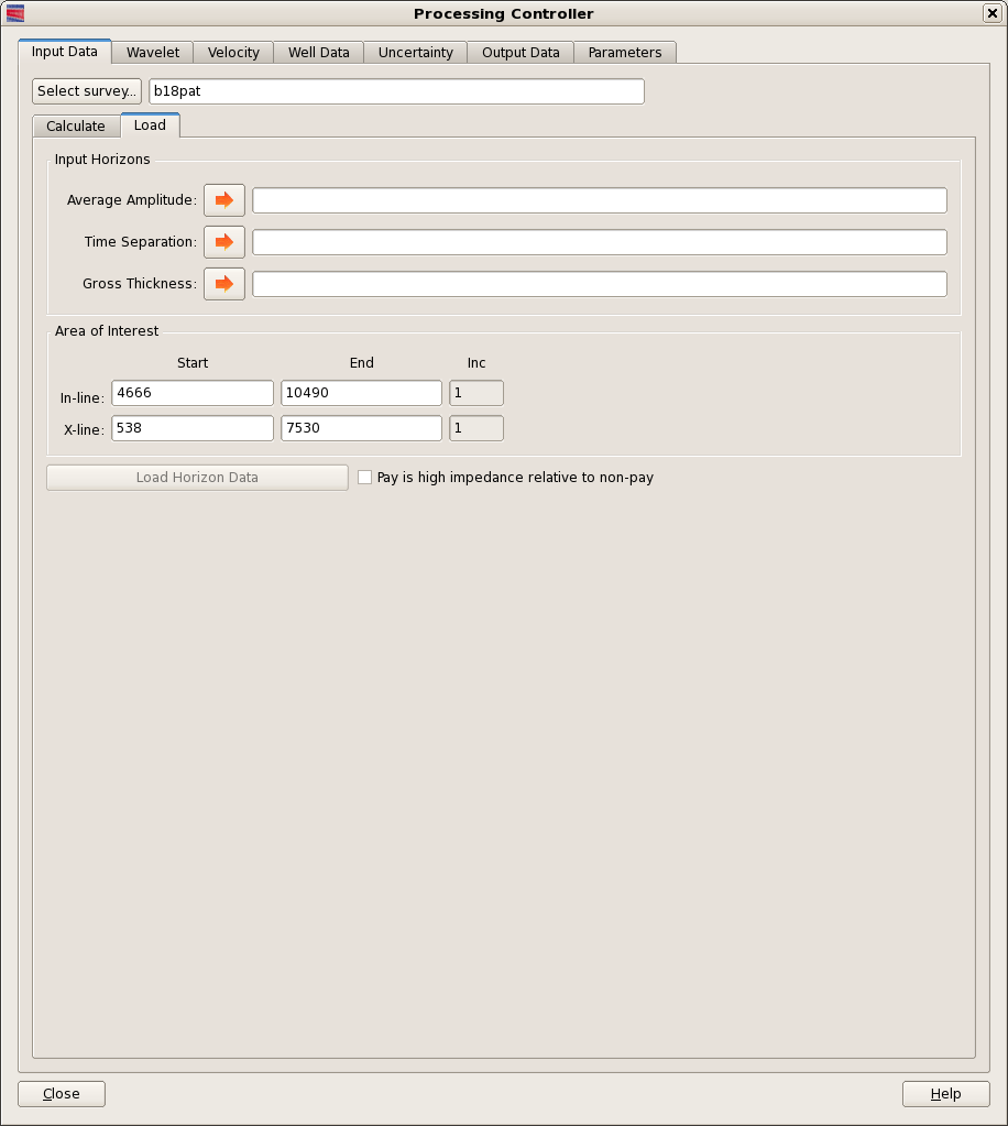
The following steps are taken in this tab:
Specify an area of interest for data loading.
The Area of Interest section will display the Inline and Xline extents of the selected survey. The values can be edited to select an area of interest.
The Inline/Xline increment is not editable by default and is for information purposes only. However, if the input horizons are decimated, with for example, in-line and cross-line increments of 2, then it is possible to make the Inline/Xline increment editable by ticking on the the Parameters tab the Inline/Xline increment Allow override box. On returning to the Input Data tab the increments will be found to be editable.
Load data from the selected horizon attributes
Once the input horizon attribute data and area of interest have been selected, the data can be loaded into SNP.
Select Pay is high impedance relative to non-pay if appropriate. This is used to screen input average amplitude values. If pay is low impedance then the average amplitude must always be negative.
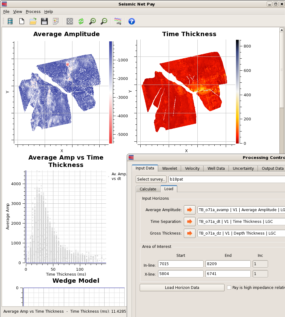
Select Load Horizon Data to load the chosen horizon attributes into the SNP application. The main window will update to show maps of average amplitude (aa), time thickness (dt), and a crossplot of aa against dt. The maps are intended only for QC purposes to check data orientation and ranges. Maps can be displayed with either X/Y coordinates or xlines on the x-axis and inlines. The coordinate orientation is controllable from the Coords toggle on the Display Options dialog when viewing grid data.
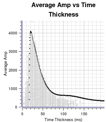
It is important that the envelope of points on the Average Amp vs Time Thickness crossplot is well defined, so it may be useful to replicate this display outside of SNP to investigate irregularities.
The wavelet tab is used to calculate the filter response that will be used within the seismic net pay calculation.
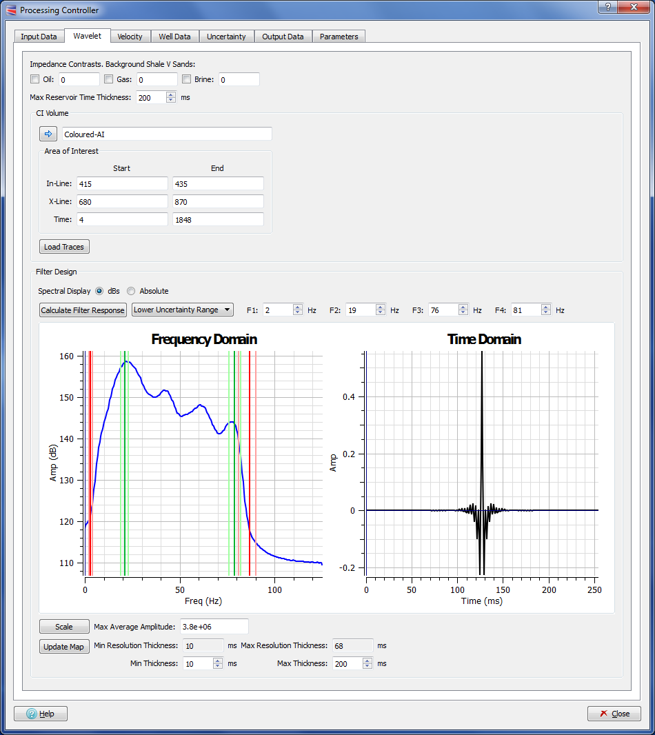
Specify Max Reservoir Time Thickness (dt) the maximum thickness over which the filter response will be calculated
Select the input Coloured Inversion Seismic Volume, which must correspond to the Volume from which the attributes were extracted.
This Seismic Volume will be used to extract an Amplitude Spectrum from which the trapezoidal filter can be designed.
Before loading the CI Volume traces, please specify your area of interest on the CI Volume, in terms of In-Lines, Cross-Lines and Time.
Specify the trapezoidal filter frequencies, F1, F2, F3 and F4. This should be the average wavelet in the seismic data at the reservoir location. The parameters should be based on a direct estimate of the CI seismic spectrum from which the attributes were extracted but allowing for the ‘alpha decay’ on the seismic impedance data.
Use the F1, F2, F3 and F4 spin-boxes to move the red and green lines (red for F1 and F4 and green for F2 and F3) to determine the trapezoidal filter frequencies F1 to F4. Use the Spectral Display radio button to switch between dBs and Absolute modes. It is recommended to select Absolute for setting the F1 and F4 frequencies and dBs for setting the F2 and F3 frequencies.
The vertical light red and light green lines that appear on the Frequency Domain chart correspond to the upper and lower filter Uncertainty frequency ranges, which are used in the Uncertainty tab. These can be adjusted by first using the combo box next to the Calculate Filter Response button to select either Upper or Lower, Frequency Ranges, and then perturbating, up and down, the values in each of the F1 - F4 spin-boxes. Note that the Calculate Filter Response button can be pressed only when the Net Pay Freq. Range option is selected. The upper and lower ranges can also be set by changing values on the Uncertainty tab.
Note that default values of zero have been set to force the user to analyse the CI data to determine the correct values for F1 to F4.
Optionally toggle on and specify the impedance contrasts for:
Background shale - oil sands (default colour red)
Background shale - gas sands (default colour green)
Background shale - brine sands (default colour blue)
If one or more of the above are specified, then the expected average amplitude response for these will be plotted on the “Average Amp vs Time Thickness” chart
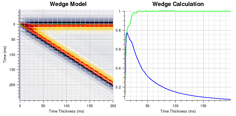
Select Calculate Filter Response to perform the internal calculation. The Wedge Model, and Wedge Calculation charts will be populated as shown below
The Wedge Model chart shows the result of passing a user defined trapezoidal filter over a narrowing low impedance model. This chart can be used to observe where the tuning thickness occurs. This is the thickness where, due to constructive and destructive interference of the upper and lower legs, the apparent wedge thickness (red line) does not become any thinner.
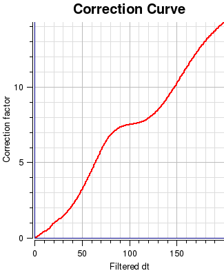
The Wedge Calculation chart shows two normalised calculations derived from the user defined wavelet. These are the seismic net pay to gross pay ratio (green), and scaled average amplitude (blue). These two data items are in turn used to calculate the values shown in the 'Correction Curve' chart that is used to remove tuning effects present in thin bedded reservoirs.
Specify Max Average Amplitude (aa) - the amplitude value corresponding to the maximum of the tuning response. This should be estimated initially from the average amplitude / time thickness crossplot. An initial estimate is provided following Calculation of Filter Response. This value may be later adjusted to optimise the well calibration.
Select Scale to plot the scaled theoretical tuning curve on the average amplitude / time thickness crossplot.
The Minimum resolution dt is the theoretical minimum time thickness of an event given the specified wavelet spectrum. The Maximum resolution dt is the time thickness at which the seismic response of a 100% net-to-gross event will split. These two values are provided for information only.
Specify Min dt. Data points having a value less than this will be set to null. Theoretically there should be no data with values less than the Minimum resolution dt but, for numerous reasons, all datasets will contain smaller values. The user should judge whether or not to decrease this value below the default to retain these data points.
Specify Max dt. Data points having a value greater than this will be set to null.
Click Update Map to register the dt range and to update the Time Thickness map to only show points between Min dt and Max dt. At this point the Poly Correction Curve is calculated and displayed on the graphics window. The curve is shown between the Min dt and Max dt. Values less than the theoretical Minimum resolution dt are linearly interpolated towards the origin. The Correction method, Look Up Table or Polynomial Fit (with a Polynomial Order) can be selected from the Parameters tab.
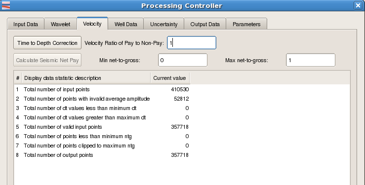
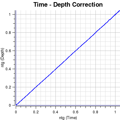
Specify Velocity Ratio of Pay to Non-Pay. This is used to convert from net-to-gross in time to net-to-gross in depth.
Select Time to Depth Correction. This displays the net-to-gross correction curve on the graphics window.
Specify Min net-to-gross.Data points having a calculated net-to-gross less than this will be set to null.
Specify Max net-to-gross. Data points having a calculated net-to-gross greater than this will be clipped to this value.
Select Calculate Seismic Net Pay to perform the internal calculation of net-to-gross (time), net-to-gross (depth) and net pay. No data is output at this stage.
Data Statistics. These will also be displayed as the internal net pay attributes are calculated. Invalid average amplitude - if pay impedance is less than non-pay impedance then the average amplitude over the reservoir interval should always be negative (and vice versa). Data points having the incorrect polarity will be set to null. A dataset containing a lot of data with incorrect polarity may indicate either non-conformance with the binary rock model assumption or incorrect picking.
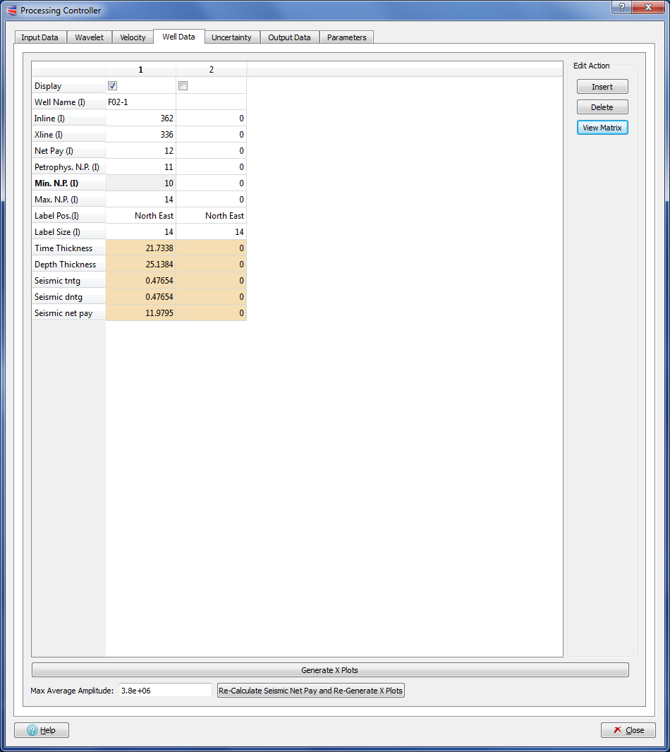
Enter Well Name, Inline, Xline and Net Pay for each well. The net pay value must be the total verticalised net pay within the reservoir interval between the seismic picks. In release V1.2 and above, you can are also enter the Petrophysical N. P. (X on the horizontal error bar), Min N.P. and Max N.P. Input columns are labelled (I). All others are output only.
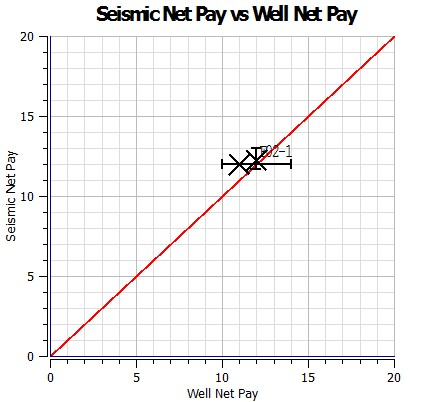
Select Generate X Plots. This will display the remaining parameter values within the table including the estimated seismic net pay. Note that you will either need to scroll or expand the window to see all the table values. The seismic net pay vs. well net pay crossplot will also be displayed in the graphics window. The crossplot points will have a vertical error bar which shows the range of net pay values from a NxN matrix around each well location. N defaults to 3.
Select a well from the table by clicking on the left hand well number column.
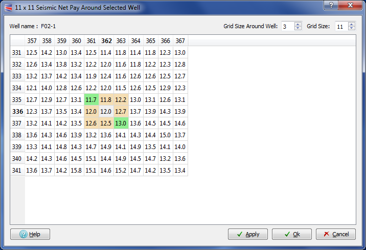
Select View Matrix. A new window will pop-up showing the calculated net pay values around the selected well. The current position of the well, the NxN matrix and the minimum and maximum values will be highlighted.
Select a new inline/xline location for the well and select OK or Apply to change the well location. The table and the crossplot will be updated. The user should refrain from making large changes to the well location without some justification.
To modify the calibration you can change the Max Average Amplitude (aa) value and press the button Re-Calculate Seismic Net Pay and Re-Generate X Plots, which will repeat all the steps done from the Wavelet to the Well tab after calculating the filter response but using the new Max Average Amplitude (aa) value. Complete optimisation may require adjustment to the wavelet specification, the calibration scalar and the well locations.
This Dialog is used to estimate the errors that can arise from calibration errors and inaccurate wavelet estimation.
The results are displayed in several charts and in tables of standard deviation values as a function of apparent thickness and seismic net-to-gross.
Click,in the selector, to calculate either Total Uncertainty or Calibration Uncertainty only.
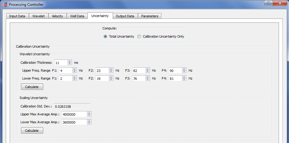
Calibration Uncertainty is in two parts
Wavelet uncertainty:
A Calibration Thickness value above the minimum thickness (Min dt) can be entered. This allows the calibration to be pinned or fixed to a gross interval where the calibration does not change (EG at the well calibration position). The upper and lower calibration curves (entered below) will cross at the specified interval.
To estimate the Calibration Uncertainty enter values for trapezoidal wavelets that are above and below the values entered in the Wavelet tab. These values will be used to calculate the upper and lower relative correction curves. The results are plotted as two curves (upper and lower) on the "Relative Correction Curves" chart.
These two correction curves are also plotted onto the "Average Amp. vs Time Thickness" chart for comparison with the P50 curve from the Wavelet tab.
The wavelet standard deviation curve (which is a function of gross interval) is calculated by first normalising the P50 wavelet (from the Wavelet tab) such that the correction curve is 1 for all gross intervals, then calculating the range between the upper and lower wavelets and dividing by two. The result is plotted on the "Normalised Std. Dev. (for ntg of 1)" chart.
The standard deviation values are plotted in a table which can be viewed by clicking the button and are displayed as a function of apparent thickness and net-to-gross.
Scaling Uncertainty:
These upper and lower max. amp. values are entered as values above and below the Maximum Average Amplitude value input on the Wavelet tab. They are used to estimate the scaling errors as a function of apparent thickness and net-to-gross. The normalised standard deviation values are calculated by, firstly, normalising the calibration scaling values such that the most likely value is 1. Then calculating the range between the upper and lower max average amplitude values and dividing by two. The result is the calibration standard deviation which is a constant.
The Calibration Uncertainty values are displayed in the chart labeled Bias Uncertainty and can be output as an Attribute Horizon in the Output Data tab.
The Amplitude Uncertainty arises from inaccurate wavelet estimation.
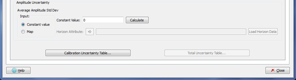
The Amplitude values can be input from either a Map or using a Constant value.
The Constant Value will be summed with the Calibration Uncertainty values to produce a chart of Total Uncertainty values. A curve of Wavelet + Scaling + Amplitude standard deviation values are plotted on the Normalised Std. Dev. chart as a function of Gross Interval and Normalised Standard Deviation. These Total Uncertainty values can be output in the Output Data tab and saved as an attribute Horizon. The Total Uncertainty values are also displayed in the Total uncertainty Table. Input the Constant Value and click the button to add the value to the Calibration Uncertainty values.
The Map should contain a set of Standard Deviation values that will be summed with the Calibration Uncertainty to produce a chart of Total Uncertainty values. These values can be output in the Output Data tab and saved as an attribute horizon. Clicking the data button will add the map values to the Calibration Uncertainty values.
The output data tab is used to choose the attributes that will contain the data calculated by the seismic net pay application.
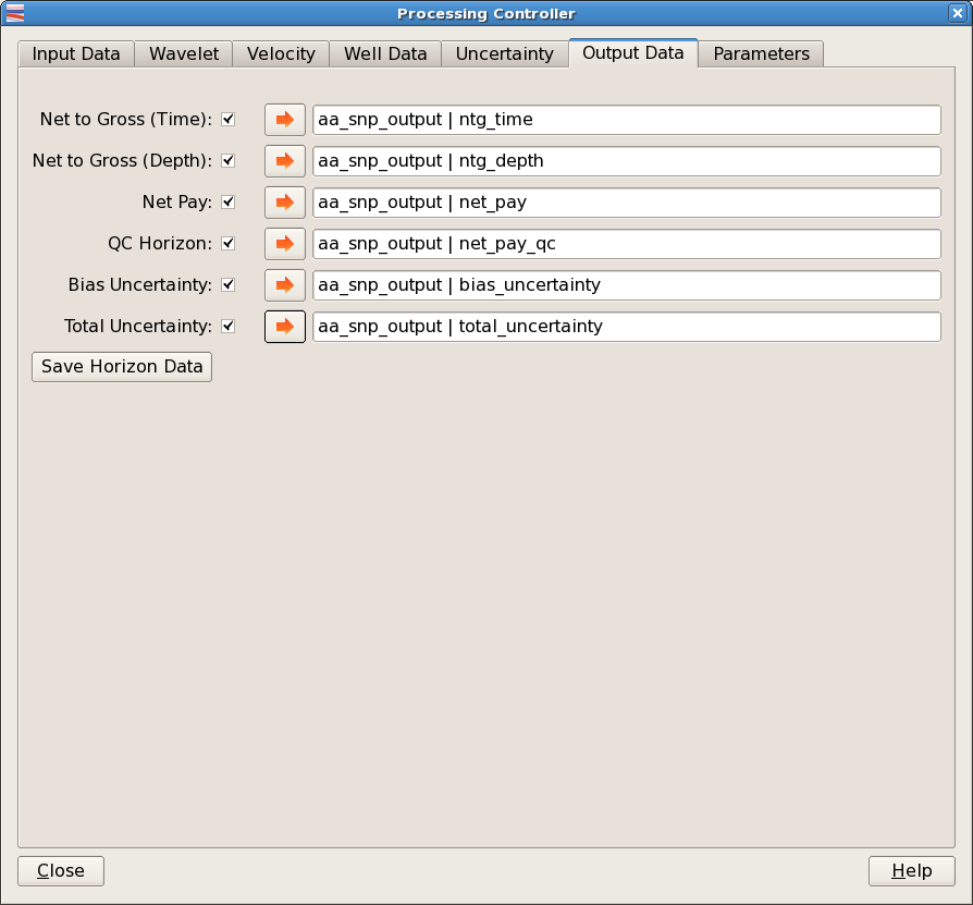
Select which attributes you wish to output. The options are:
Net-to-gross (time)
Net-to-gross (depth)
Net pay
QC horizon
Bias Uncertainty
Total Uncertainty
Select horizons for output by checking the check-box. The Bias Uncertainty and Total Uncertainty attributes are only available for output if the Uncertainty tab has been used. Attributes 1 and 2 will be the same if the Velocity Ratio of Pay to Non-Pay is equal to 1.Net Pay is equal to the product of Net-to-gross (depth) and Gross Thickness. The QC horizon indicates the status of each data point. It can take one of three values:
Data has a dt value greater than Min dt and less than Max dt (ie good data).
Data has a dt value less than Min dt. The output data will therefore have been set to the Undefined value.
Data has a dt value greater than Max dt. The output data will therefore have been clipped to Max dt.
To get detailed information about how to select the output horizon attributes, go to the section Select Output Horizon Attributes.
When all required attributes have been specified, the Save Horizon Data button on the Output Data tab will become active. Click this button to save the attributes.
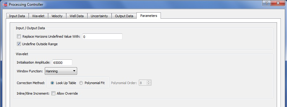
The Parameters tab can be used to affect the operation of the processing controller by a altering a number of settings:
Initialisation Amplitude: An amplitude scalar value used in the calculation of the tuning curve from the wedge model and input filter.
WindowFunction:. The type of smoothing, Hanning or Hamming - Tukey, applied to the corners of the frequency spectrum input in the Wavelet tab.
Correction Method: The method used to recalculate the Correction Curve after Self-Calibration, either by Look-Up table to by using Polynomial Fit coefficients.
Inline/Xline increment: If Allow override is selected, the 'increment' field on the Input Data tab will become activated. This will allow the user to overrided the default sampling interval for input horizon data.
Output Options: If Undefine Outside Range is selected, values of dT calculated to be outside of the range Min dT to Max dT will cause values of net-to-gross (time), net-to-gross (depth) and net pay to be set to the Undefined Value. No data is output at this stage.
Undefined Horizon value: If this option is selected, the number entered will be used to represent data values in the horizon data (both Input and output). No data is output at this stage.
This section describes how to select input seismic volumes that will used in the calculation of horizon attributes.
Press the ![]() button next to the text 'AI Volume' to display the 'Select Volume' dialog. This shows a list of available seismic volumes. A Filter is provided to reduce the list to a manageable size for projects with many seismic volumes.
button next to the text 'AI Volume' to display the 'Select Volume' dialog. This shows a list of available seismic volumes. A Filter is provided to reduce the list to a manageable size for projects with many seismic volumes.
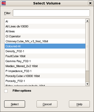
The image in the figure above shows the "Select Volume" dialog for selection of a seismic volume without a list filter. Use the Filter to create a shorter list.
Select the volume you require for your SnpQt analysis, and then press the Select button. You should see the details of the selected volume appear next to the arrow pressed.
This section describes how to select input horizon attributes that will be used in the net pay calculation.
To select an input horizon and attribute, press the ![]() button next to either 'Average Amplitude', 'Time Separation', or 'Gross Thickness' to display the 'Select Horizon Attribute' dialog.
button next to either 'Average Amplitude', 'Time Separation', or 'Gross Thickness' to display the 'Select Horizon Attribute' dialog.
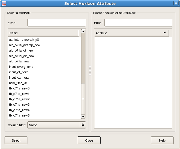
This dialog shows a list of available horizons, and for each selected horizon, the available attributes. The list of available attributes is updated when a horizon is selected, as shown below:
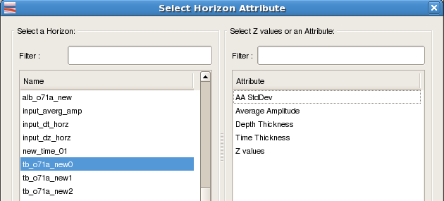
The attribute can be selected by clicking on it, and then pressing the 'Select' button. or by double clicking the desired attribute. In either case, the combination of selected horizon and attribute will be shown in the input data tab:

Note that when a horizon/attribute is selected by double clicking, the Select Attribute dialog remains open for the attribute of the next required horizon to be selected. So in the view above, where 'Average Amplitude' has been selected, when the next horizon atribute is double clicked, it will appear in the 'Time Separation' field.
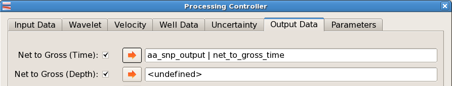
This section describes how to select output horizon attributes that will be used in the net pay calculation.
To select an output horizon and attribute, press the ![]() button next to the desired attribute to display the 'Select Horizon Attribute' dialog.
button next to the desired attribute to display the 'Select Horizon Attribute' dialog.
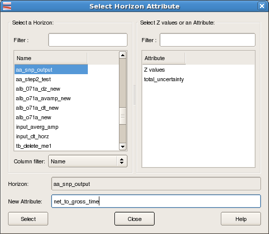
This dialog shows a list of available horizons, and for each selected horizon, the available attributes. The list of available attributes is updated when a horizon is selected.
The user can either select an existing attribute in this way, in which case it will be overwritten when saved, or can enter a new attribute in the 'New Attribute' text field. When a selection has been made, press the 'Select' button, and the chosen horizon/attribute name will appear by the ![]() button.
button.
Like the case with input horizons, horizon/attributes can be selected by double clicking. This will populate the attribute next to the originally clicked ![]() and move the input focus to the next attribute type. This mechanism can be used to rapidly specify all required output attributes if existing horizon/attribute combinations are required.
and move the input focus to the next attribute type. This mechanism can be used to rapidly specify all required output attributes if existing horizon/attribute combinations are required.