The SFE utility can best be described by consideration of the diagram in figure 1 below.
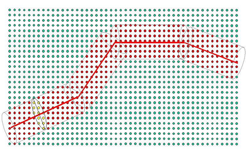
This diagram shows colour coded symbols which represent the processed bin locations of a sample 3D seismic survey. The heavy weighted red line shows the digitized traverse requested by the User. In this example, the traverse is built up of four line segments. Parallel to each line segment and either side of it are two grey colour coded lines. These lines, together with the outer boundary of the aperture at either end of the line segments, determine which bins will be used in the processing of a given line segment. The aperture can be either an ellipse or a rectangle, but for the purpose of this discussion we shall treat the aperture as being an ellipse. The bins, within this bounded area, are colour coded red. The aperture in the middle of segment 1 shows an example of a traverse trace being processed. At a given traverse output trace location, an aperture is effectively superimposed over the 3D seismic survey. The traces at the 3D bin locations that are within the boundary of the aperture are used to construct a 3D traverse trace at the centre of the aperture. In the diagram, these bins have been colour coded yellow. Each traverse trace is processed in turn to build up the traverse trace by trace. For database and resource efficiency, it will be preferable to treat each line segment separately. Traces within the aperture are read and stored within virtual memory. A trace management facility has been built into the utility so that input traces needed by the next 3D traverse trace, as the aperture is moved up, are not lost. This reduces the database I/O events. Further information on this can be found in the Appendix A - Aperture Geometry.
The User must supply the coordinates for each line segment. This can be done in one of two ways. Either manually input or via a polygon from the database. The recommended, and by far the easiest and less error prone, is the polygon method. Here the User creates a Traverse whilst running SeisWorks 3D. The knee points of the Traverse are output to a point file. Other control data (e.g. Auto swath width, size of major and minor axes of the ellipse) are normally supplied via the Aperture Geometry Dialog.