This section describes how you can vary various parameters to improve the Spectral Blueing operator.
SsbQt is data driven, so once the data is identified and loaded then a Spectral Blueing operator will immediately be available for saving. This makes the Spectral Blueing analysis very easy for the end user. However, the resulting operator may not be optimum. Therefore, it will frequently be necessary to perturb various design parameters to produce the optimum Spectral Blueing operator. The various charts within the main window are used to help you produce the ideal Spectral Blueing operator for your data. Below is a description of the primary parameters used to design the Spectral Blueing operator. Additional parameters can be found under the "Advanced Controls" dialog.
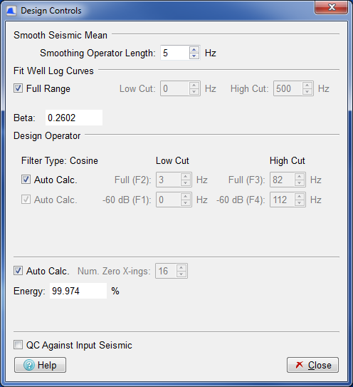
The Design Controls dialog is split into three groups: Smooth Seismic Mean, Fit Well Log Curves and Design Controls. The following three sections describe these groups.
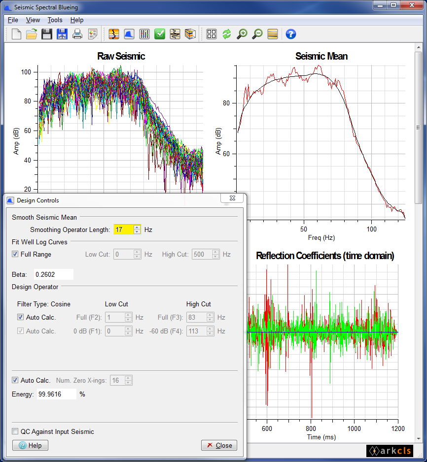
The only parameter in this group is the Smooth Operator Len (Hz). This spinbox controls the length of the smoothing operator used in the smooth mean algorithm that is applied to the seismic mean spectrum. It has a range of 1 - 1/5th nyquist and by default it is set to a value of 1/25th nyquist. View the chart named "Seismic Mean" whilst changing the value in the spinbox to see the effect of this parameter. The aim here is to iron out high frequency amplitude variations as we are only interested in the global shape of the seismic spectrum. The image in the figure above shows the smooth mean spectrum (black) overlaying the mean spectrum (red). Here the Smoothing Operator Len is set at 17Hz.
This checkbox item allow you to control whether curve fitting is performed on the full range. The spinbox controls in this group are the primary parameters used for principal curve fitting.
Full Range checkbox (checked) - default on the distributed template
In this mode, curve-fitting is performed on the global spectrum and will be performed on the "Full Range". The Low Cut and High Cut for Fit Well Log Curves will be desensitised.
Full Range checkbox (unchecked)
In this mode, curve fitting consists of three curves "Below Principal", "Principal" and "Above Principal". The intersection between the "Below Principal" and the "Principal" curves is at the "Low Cut" point. The intersection of the "Principal" and "Above Principal" curves is at the "High Cut" point. The "Low Cut" spinbox is the Minimum Fit Frequency of the principal curve and the "High Cut" spinbox is the Maximum Fit Frequency of the principal curve. The other curves outside this range are generated in accordance with the controls on the "Frequency Domain" tab on the "Advanced Controls" dialog.
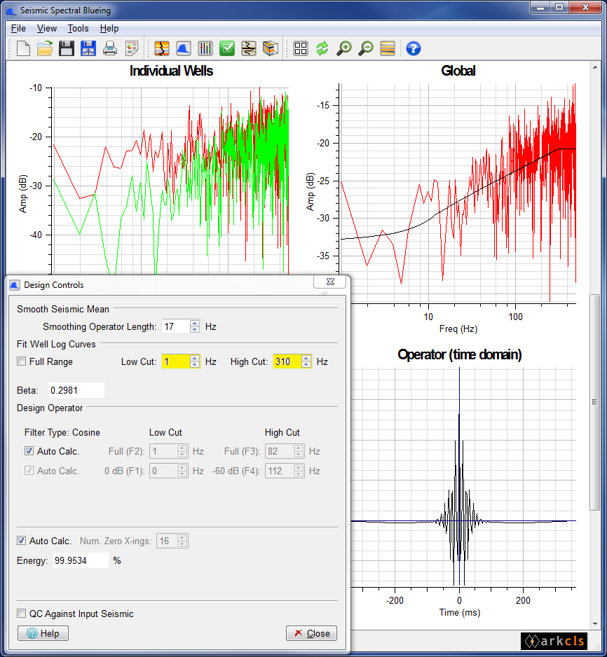
Low Cut: This spin box allows you to specify the minimum frequency that the curve fit algorithm will attempt to fit for the principal curve. By default, this is set to zero Hz. However, if including lower frequencies is not of any concern to you or you wish to additionally use a low frequency curve or linear horizontal low frequency section, then setting this to a higher value can often result in a better curve fit over the frequency range of interest.
High Cut: This spin box allows you to specify the maximum frequency that the curve fit algorithm will attempt to fit for the principal curve. By default, this is set to the nyquist frequency. However, if including higher frequencies is not of any concern to you or you wish to additionally use a high frequency curve or linear horizontal high frequency section, then setting this to a lower value can often result in a better curve fit over the frequency range of interest.
Curve fitting is updated immediately the "Low Cut" control, "High Cut" control or the "Frequency Domain" controls on the "Advanced Controls" dialog are changed. In this case we have defaulted the Low Cut to zero Hz and have set the high cut to 300Hz. The Above Principal curve fit is horizontal.
At any time you can curve fit to the full spectrum 0 Hz - nyquist by toggling on the "Full Range" checkbox within the "Fit Well Log Curves" group.
The field Beta displays the value of this key curve fitting parameter which can be changed on the "Advanced Controls" dialog.
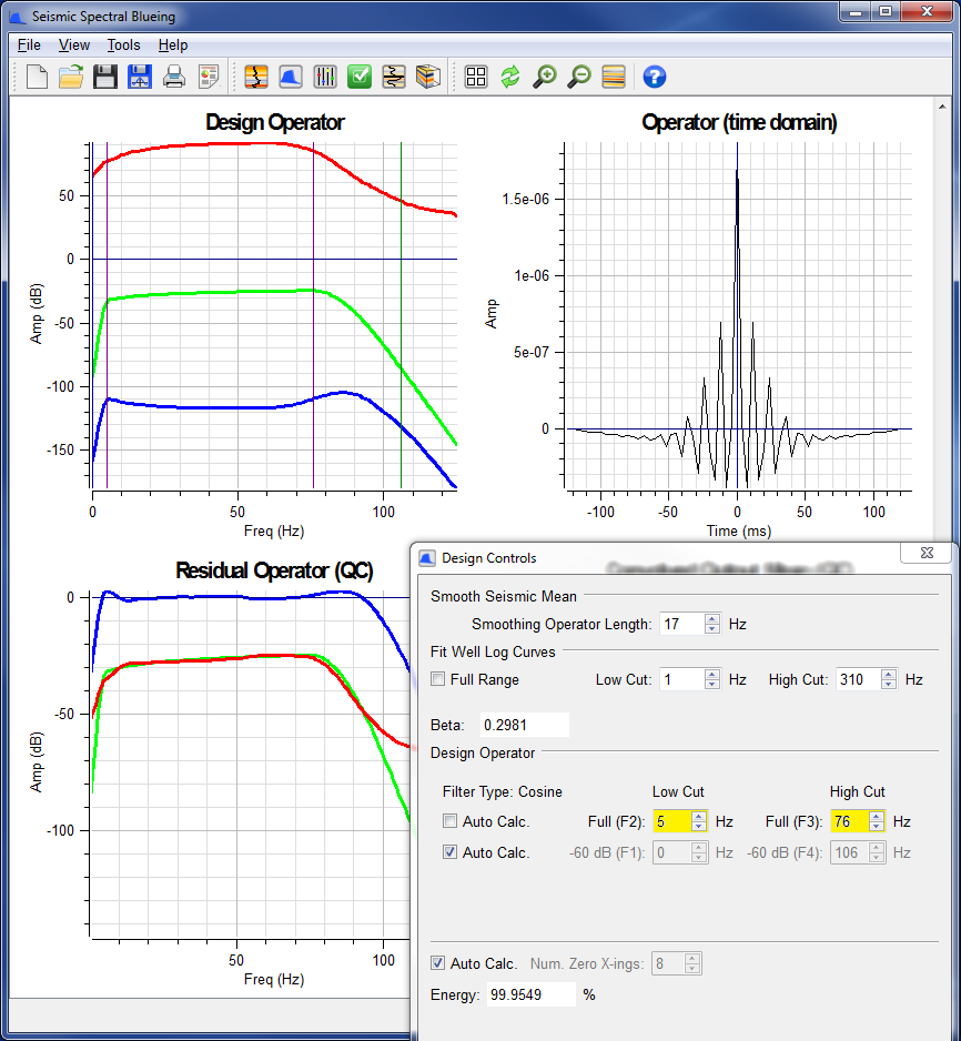
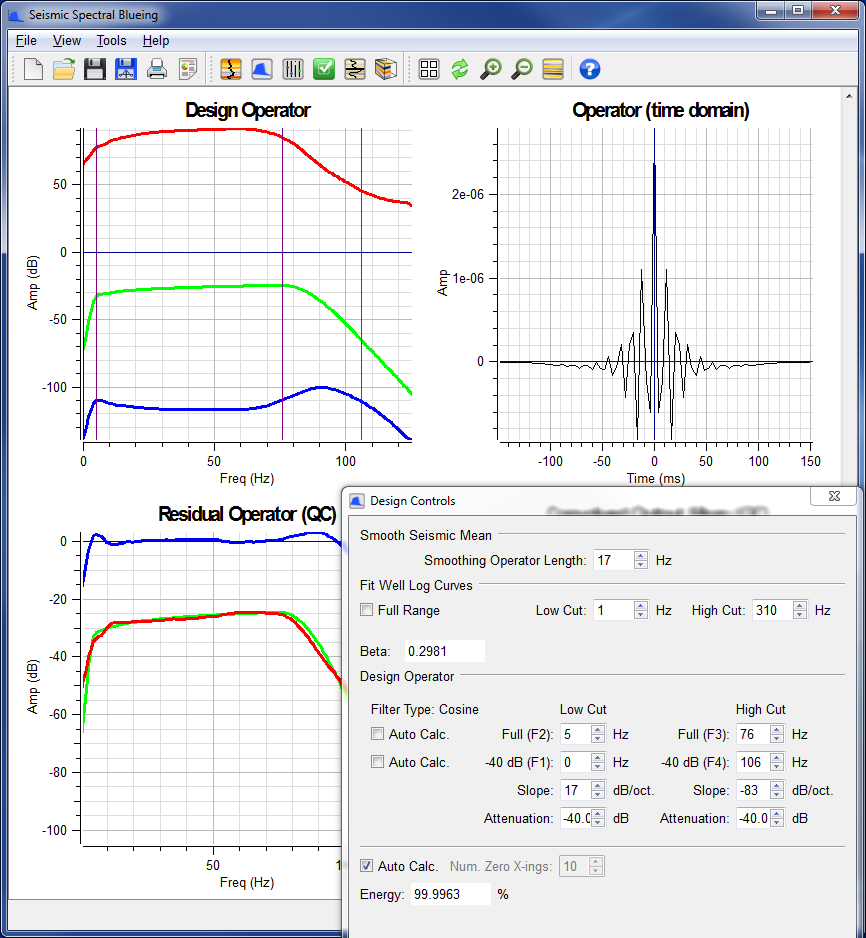
The "Design Operator" group provides controls which allow you to perturb how the Spectral Blueing operator spectrum is generated. Specifically, it allows you to adjust the bandwidth of the designed operator. Normally, the default is that the bandwidth is automatically calculated. The "Design Operator" chart displays three spectra. The first spectrum is the band limited curve fit (green curve), the second spectrum is the smooth seismic mean (red curve) and the third spectrum is the Spectral Blueing operator (blue curve).
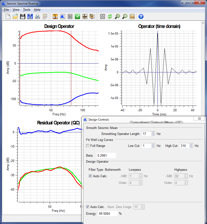
There are two methods for filtering the operator, Cosine and Butterworth.
The top checkbox controls whether the "Low Cut" and "High Cut" (i.e. design operator bandwidth) values are automatically calculated.
Upper Auto Calc. checkbox (checked) - default on the distributed template
In this mode the design operator bandwidth is automatically calculated
Upper Auto Calc. checkbox (unchecked)
In this mode you can manually set the "Low Cut" and "High Cut" spinboxes.
this control will be sensitised allowing you to adjust the low cut to optimise the Spectral Blueing operator. Using the "Residual Operator (QC)" chart will help. The objective here is that the residual operator should be essentially flat and centred around 0 dB within the bandwidth.
this control will be sensitised allowing you to adjust the high cut to optimise the Spectral Blueing operator. Using the "Residual Operator (QC)" chart will help. As with the Low Cut, the objective is that, the residual operator should be essentially flat and centred around 0 dB within the bandwidth.
The lower checkbox allows you to control the slopes on the derived operator. This checkbox is only sensitised if you are manually setting the design operator "Low Cut" and "High Cut" (i.e. the top Auto Calc checkbox is unchecked).
Lower Auto Calc. checkbox (checked) - default on the distributed template
In this mode, the attenuated down point (default: -60 dB) is at 0 Hz on the low size with the attenuated down point (default: -60 dB) 30 Hz above the High Cut value on the high side.
Lower Auto Calc. checkbox (unchecked)
In this mode you can manually specify the frequency of the attenuated down point both on the low and high sides.
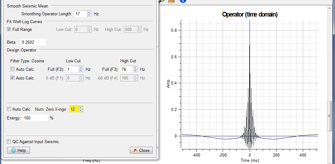
Notice that the four filter frequency points F1, F2, F3 and F4 are marked on the chart as narrow vertical lines. These move position as the filter frequencies are changed. See the Design Operator chart in the figure above.
 ...
...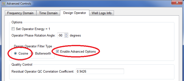
The Advanced Controls allows the user control over the amount of attenuation at the F1 and F4 filter points. The default attenuation value of -60dB is considered too high for modern broad-band seismic data.
To enable the additional advanced controls check the Enable Advanced Options check-box in the "Design Operator" tab in the Advanced Controls window. See the right hand figure in the figures above. The additional controls become available after the "Auto Calc. check-box for filter points F1 and F4 is un-ticked.
There are four additional controls, and . These parameters allow control over the amount of slope in dB/octave between F1 and F2 and also between F3 and F4, which in turn, controls the amount of attenuation at F1 and F4 respectively.
Altering the Slope value will automatically recalculate the Attenuation value and vice-verca. Changing either of the F1 or F2 values (or F3 and F4) will automatically recalculate the Slope with the Attenuation staying fixed.
 ...
...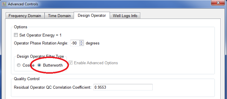
The Butterworth filter is excellent for applying a straight forward band-pass filter because the degree of filter roll-off can easily be controlled while leaving the centre frequency unchanged. The shape of the filter is controlled by essentially only four parameters: Low and Highpass Frequency and Low and Highpass Order.
To switch to use a Butterworth filter click the Butterworth option in the Design Operator Filter Type in the "Design Operator" tab in the Advanced Controls window. See the right hand figure in the figures above.
The checkbox controls whether the Low and Highpass Frequency values are automatically calculated.
Auto Calc. checkbox (checked) - default on the distributed template
In this mode, the Low and Highpass Frequency values are automatically calculated.
Auto Calc. checkbox (unchecked)
In this mode the Low and Highpass Frequency values can be manually specified to optimise the operator. These frequecy values are applied at -3dB or half power. Using the "Residual Operator (QC)" chart will help find the optimum frequencies. The objective here is that the residual operator should be essentially flat and centred around 0 dB within the bandwidth.
Lowpass and Highpass controls are available to control the roll-off slopes of the filter separately at both the lowpass and highpass ends. A lower number results in a shallower slope and a higher number increases the slope. Higher Order values will result in a more sharply designed filter but will result in more side-lobes or ripples being introduced into the output data.
The bottom checkbox in the Design Operator block controls whether the "Num. Zero X-ings" (i.e. time domain operator truncation) value is automatically or manually calculated.
Bottom Auto Calc. checkbox (checked) - default on the distributed template
In this mode, the truncation of the time domain Coloured Inversion operator will be automatically determined. This is controlled by a parameter which sets the percentage of energy captured. The percentage of energy captured template parameter is currently set at 99.9%. If the minimum level of automatic truncation were to take the energy captured below this threshold, then no truncation is performed and 100% of the energy would be captured. It is planned that future versions of SsbQt will allow you to set template (default) parameters. It is sometimes desirable to alter the amount of truncation applied in order to reduce the length of long tails of very small sample values or to include additional samples of significant value.
Bottom Auto Calc. checkbox (unchecked)
In this mode, the spinbox must be set manually. This allows you to adjust the length of the time domain operator in steps of zero crossings. It is desirable to have the operator truncate to a sample point close to a zero crossings point as it reduces anonymous side effects which might be introduced when the operator is applied.
A read only field to the right displays the percentage of energy captured as you adjust the number of zero crossings.
This checkbox control, if checked, allows you to perform the QC against the original set of random seismic traces instead of the alternative set of random seismic traces.
QC Against Input Seismic checkbox (unchecked) - default on the distributed template
In this mode, the calculation of the Spectral Blueing operator is performed using the original set of random seismic trace (listed on Select Input Data dialog -> Input Seismic tab -> Input tab). The QC of the Spectral Blueing operator is performed on the alternative set of random seismic traces (listed on Select Input Data dialog -> Input Seismic tab -> QC tab).
QC Against Input Seismic checkbox (checked)
In this mode, the calculation of the Spectral Blueing operator is again performed using the original set of random seismic trace (listed on Select Input Data dialog -> Input Seismic tab -> Input tab). However, the QC of the Spectral Blueing operator is performed on the same set of random seismic traces (listed on Select Input Data dialog -> Input Seismic tab -> Input tab).