SciQt integrates with various third party data repositories. This should be transparent to you and is dependent on how the software was launched. To use the Coloured Inversion application to design an operator, it is first necessary to analyse the seismic and well data spectra. This is achieved by loading some seismic trace data and well log impedance data in time. Pop up the "Select Input Data" dialog by either clicking the menu item under the menu bar or by clicking the  icon.
icon.
The table below shows both tabs of the Select Input Data dialog with an example of data selected for Coloured Inversion operator design. Seismic Coloured Inversion is data driven which means that the complete analysis and design of the operator (or as far as possible) are performed as soon as the data is selected/loaded or updated.
With the "Select Input Data Dialog" displayed, click the "Input Seismic" tab (default) to select the input seismic data to be used. The SciQt will connect with various data repositories depending on the environment in which the Coloured Inversion software is being run. It attempts to do this in such a manner that the Geoscientist need know only minimal information to be able to connect seamlessly with the seismic database. However, as data repositories from third party vendors use different techniques to store data, there will inevitably be some differences with the specific seismic selection mechanism.
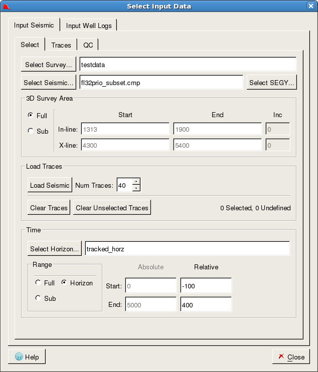
The figure above shows the Select Input Data dialog for seismic selection. Whilst this dialog might look busy you should find it easy to provide the required parameters if you follow the steps below.
Selected Survey
The push button allows you to pop-up a selector dialog allowing you to select a seismic survey. Note this selector is only seen when SciQt is run in an OpenWorks R5000 environment. When in a 2003.12 environment this selector will not be seen.
Selected Seismic
The push button allows you to pop-up a seismic volume selector allowing you to select a seismic volume.
3D Survey Area
Trace data for the spectral analysis can be selected from either the full 3D survey area or from a sub-area using the In-line/X-line Start and End input fields. By default the full area is selected.
Load Seismic
Clicking the button causes the random set of traces over the 3D Survey Area to be loaded (Input tab) for spectral analysis. At the same time an alternative set of traces are loaded (QC tab) which are used to QC the derived operator.
Set Time Range
The aim is to design a Coloured Inversion operator for the zone of interest (target). It is therefore desirable to time gate the selected traces prior to generating trace spectra. Ideally, you should use a well defined interpreted horizon in the target zone to guide the seismic trace time gate. In this manner, the various gated traces should have sample values over a similar geology.
Click to pop up a horizon select dialog, then select horizon and then click button to return.
Click in the radio button and specify the Relative Start and Relative End values. A negative number is a relative time above the horizon (i.e. shallower) and a positive number is a relative time below the horizon (i.e. deeper). The aim is to select a time gate trace which has a gate length within the range 500 - 1000 msec. The user supplied values here are accepted and the chart area updates when you do any of the following: press Return key, press Enter key, press Tab key, or mouse click on a different widget.
Note: If no horizon data is available and if seismic volume is relatively flat, then using an absolute sub range would be adequate. If it is not flat or the geology changes considerably over the 3D survey area then the selection of a smaller 3D Survey Area might be desirable.
With the "Select Input Data" dialog displayed click the "Input Well Log" tab to select the well log data to use. The SciQt software supports reading acoustic impedance in time from ASCII files or by connection to a well log data repository. Here, we shall assume you will normally wish to obtain data from OpenWorks well log data repository and we will describe this route. If you wish to load from ASCII files then please refer to the full User Manual. Currently, GeoFrame users have no option to load AI data via a database route.
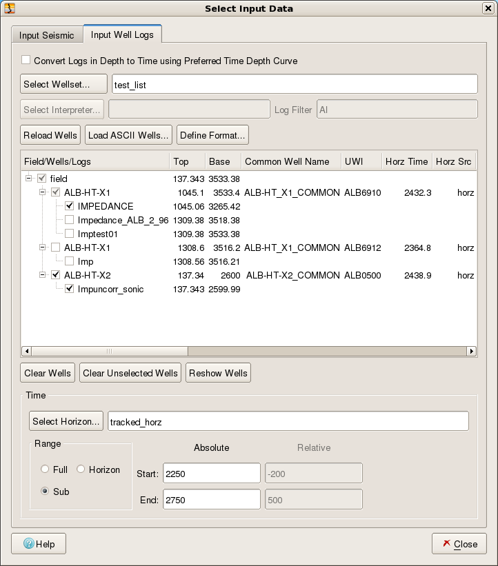
The list below shows the steps to generate well log spectra:
Load Wells
Click the push button to pop-up a dialog to allow you to select a Wellset. With your chosen Wellset, acoustic impedance log curves in time will automatically be loaded from OpenWorks. It is assumed that acoustic impedance log curves in time will have the characters "imp" (upper or lower case) somewhere within the curve name field or "impedance" (upper or lower case) somewhere in the remark field. If, for a given well, the AI log curve doesn't meet the assumed naming convention, then the user can still select an acoustic impedance log curves manually. This is achieved by right clicking on the well name after first attempting to load the wells automatically. Note the push button will change to a push button after the initial automatic selection.
Right clicking will pop-up a menu item. Selecting this item will pop-up a dialog which lists the available logs allowing you to choose an AI log curve however it is named.
This data in the time domain can be displayed on one or more Main Window charts. By default, the AI data (in time) is displayed on the "Log Input (time domain)" and "Log Input Detrend (time domain)" charts. As each AI log curve is loaded its amplitude spectrum is also immediately calculated and displayed by default on the "Individual Wells" chart.
The central area of the "Select Input Data" dialog (Input Well Log tab) shows the available acoustic impedance log curves for each well. You can deselect wells and/or log curves by clicking on the appropriate .
Set Time Range
Again, our aim is to design a Coloured Inversion operator for the zone of interest (target). It is therefore desirable to time gate the selected traces prior to generating well log spectra. Ideally, you should use a well defined interpreted horizon in the target zone to guide the well log trace time gate. In this manner the various gated traces should have sample values over a similar geology.
Click to pop up a horizon select dialog, select horizon and then click button to return.
Click in Range radio button and specify the Relative Start and Relative End values. A negative number is a relative time above the horizon (i.e. shallower) and a positive number is a relative time below the horizon (i.e. deeper). The aim is to select a time gate which has a gate length within the range 500 - 1000 msec. The user supplied values here are accepted and the chart area updates, when you do any of the following: press Return key, press Enter key, press Tab key or mouse click on a different widget.
With the seismic and well data loaded the SciQt application will complete all the various steps to generate a Coloured Inversion operator. However, with this data driven approach the initial derived Coloured Inversion operator may not be optimum. As such, it may be necessary for you to perturb some of the design parameters before saving the operator. Apart from controlling the desired data and data ranges, all other design parameters are accessible via "Design Operator Dialog" (see section below) and the "Advanced Controls" dialog