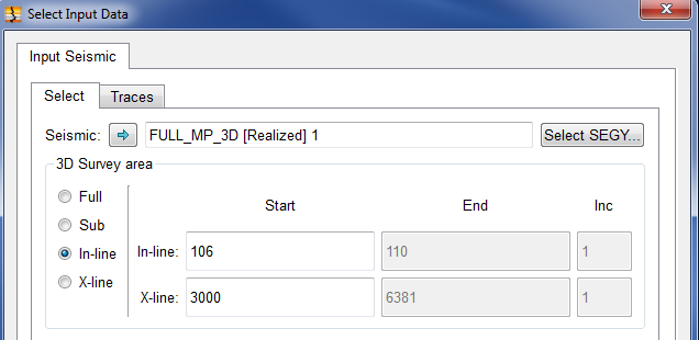
This section provides a Select Sesimic... button which will allow you to pop-up a seismic selector dialog. This section also allows you to specify the In-line, Cross-line or 3D Survey Area to be used to retrieve trace data for SGS analysis.

Figure 4.18. Select Input Data dialog (Input Seismic Tab)

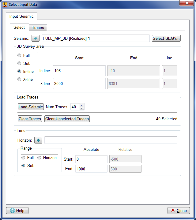
With the seismic data selected, it is usually desirable to define either sequential traces from an in-line or cross-line, or random traces from a sub-area. This is achieved by clicking either the In-line, X-line or Sub buttons from the 3D Survey Area radio button group. Following this, the user would specify the in-line and the starting cross-line to read sequential traces from, the cross-line and the starting in-line, or the sub area using the Start In-line, End In-line, Start X-line and End X-line edit boxes. Finally, the number of traces is specified and the Load Seismic button is clicked. When In-line or X-line these traces are sequential from the starting trace, or random in the case of a Full or Sub area.

With the seismic data volume selected you can now load a set of traces to be analysed. Here you can optionally choose to select traces from the full 3D survey area or sub 3D survey area. This is achieved using the 3D Survey Area radio button group as follows:

Typically you would select sequential traces from an in-line or cross-line, or maybe random traces from a sub-area. This is achieved by clicking either the In-line, X-line or Sub buttons from the 3D Survey Area radio button group. Following this, the user would specify the in-line and the starting cross-line to read sequential traces from, the cross-line and the starting in-line, or the sub area using the Start In-line, End In-line, Start X-line and End X-line edit boxes. Finally, the number of traces is specified and the Load Seismic button is clicked. When In-line or X-line these traces are sequential from the starting trace, or random in the case of a Full or Sub area. This is then followed by you clicking the Load Seismic button to load a set of traces. The software also enables you to select trace data from multiple in-lines, cross-line or sub-areas. This is achieved by specifying another trace range and clicking the Load Seismic button again. The goal is to generate seismic trace spectra which is a good representation of the area as a whole. If you attempt to specify an area which is outside of the available area then a warning message will be issued when you attempt to load seismic traces by clicking the Load Seismic button. You will also get an error message if you set an area which would not allow enough unique traces for the Num. Traces requested.

Figure 4.19. Loading Seismic Data

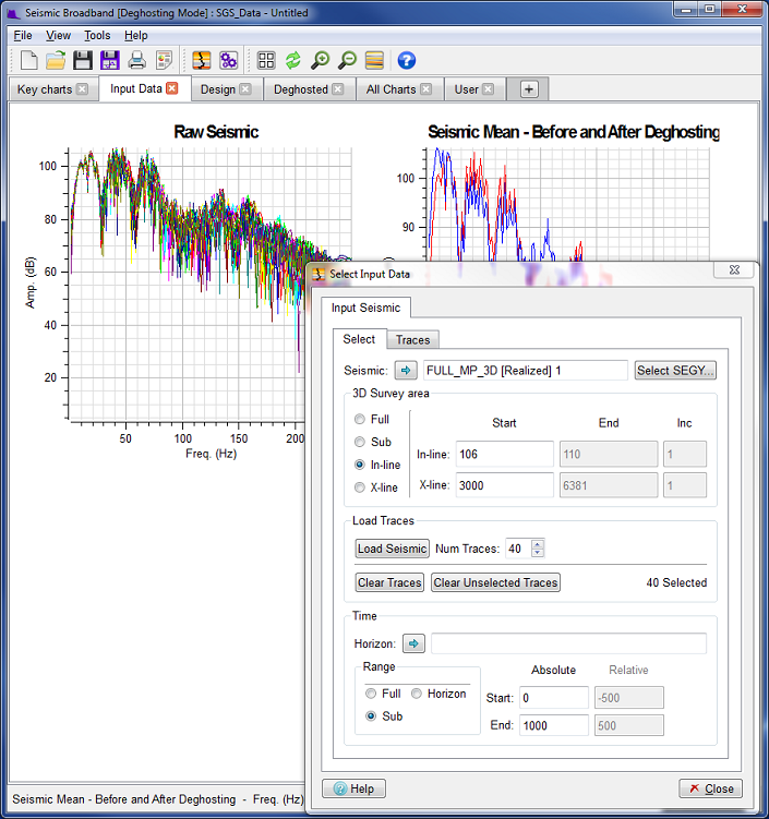
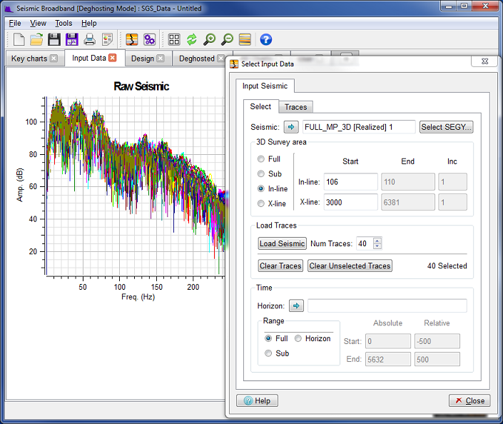
The image in the figure above shows the application main window with Select Input Data Dialog superimposed. The Raw Seismic spectra resulting from clicking the Load Seismic button on the "Select Input Data Dialog" (above left) with Num. Traces set to 40 and traces defined by:

In-line: 106

Starting X-line: 3000

By default, all loaded traces are used in the spectra calculation and contribute to the Seismic Mean Spectrum. However, you can remove a given trace from the SGS analysis by deselecting it via the Input list. Deselection of a trace is simply achieved by unchecking the checkbox within the list. If you want to completely remove the deselected trace you click the Clear Unselected Traces button. Alongside each trace on the Input list, are various properties associated with the trace. These include Trace Id (or trace label), In-line, X-line, RMS Amp, RMS Err, Horz Time. The RMS Amp property is derived from the input seismic trace, whereas the RMS Err property is derived from the trace spectrum. The latter can be considered as a "goodness of fit" parameter as it compares trace spectrum with the smooth mean trace spectrum. So for RMS Err, the smaller the number the better the fit. Loaded traces, by default, are sorted by Trace Id. However, you can sort the list of traces using one of the other properties. This is easily achieved by clicking the column header on the Input list. So, for example, if you want to sort by RMS Amp in ascending order, you click the RMS Amp header label. To sort in descending order you click the RMS Amp header label again. You can also change the position of the property columns. This is simply achieved by clicking and holding on a property header then dragging the property header to its new position.

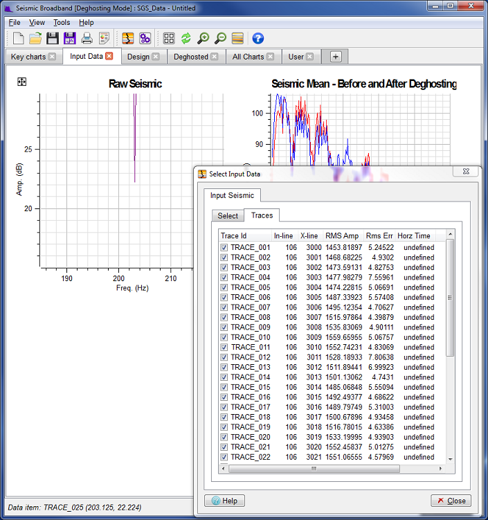
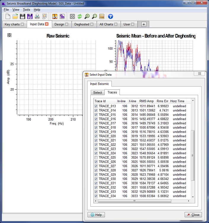
The image shows the result of clicking the Load Seismic push button. Here 40 traces have been randomly loaded and immediately displayed in the "Raw Seismic" chart within the application main window. Also visible is a portion of the "Select Input Data Dialog" showing the trace list on the "Input" tab sorted by ascending RMS Amplitude values.

Figure 4.20. Clearing Seismic Data

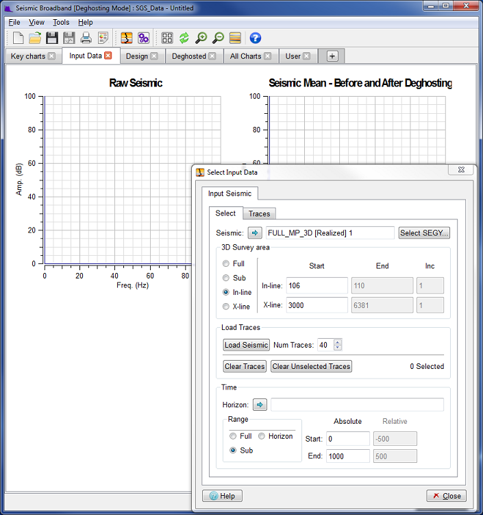
The image in the figure above shows the result of clicking the Clear Traces push button. Clear traces removes all traces previously loaded to memory and has the immediate effect of removing this data from the "Raw Seismic" chart within the application main window.

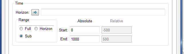
Specifying the time range (gate) is an important step. Ideally, you should choose a time gate in the range of 500 - 1000 msec which should be over the zone of interest. You can set the Time Range mode in one of three ways via the "Range" radio button.

Of the three options the Horizon Range mode is the preferred mode since it allows the gate to follow the geology and should, with a well interpreted horizon in the target zone give, in theory, trace spectra which are more closely matched.

Figure 4.21. Modifying Seismic Time Range (Full)

The image in the figure above shows the application main window with Select Input Data Dialog superimposed. Here, "Full" (full trace range) has been selected for the Range radio button. This mode is rarely used since our goal is to design the operators over the zone of interest. This will optimise the process over that zone. However, it does allow you, although insensitive, to see the start and end times of the entire trace.

Figure 4.22. Modifying Seismic Time Range (Sub)

The image in the figure above shows the application main window with Select Input Data Dialog superimposed. Here, "Sub" (sub trace range) has been selected for the Range radio button. In this mode the Absolute Start time and the Absolute End time Line Edit fields will be sensitised. This allows you to specify a time gate for the zone of interest.

Figure 4.23. Modifying Seismic Time Range (Horizon).

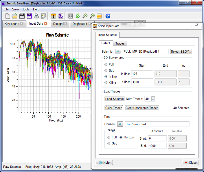
The image in the figure above shows the application main window with Select Input Data Dialog superimposed. Here, "Horizon" (horizon relative trace range) has been selected for the Range radio button. In this mode the Relative Start time and the Relative End time Line Edit fields will be sensitised. This allows you to specify a time gate for the zone of interest. Typically you would specify a time gate which would give you a time range between 500msec and 1000msec. Specifying the Start and End times here are relative to a geologic horizon. A negative number represents time above the horizon whereas a positive number is a time below the horizon. The time gate can be either above, below or span the horizon.

Occasionally, it is necessary to remove one or more poor spectral traces which contribute to the generation of the mean spectra. This is easily achieved by identifying problem spectral traces from the chart and deselecting these traces from within the Select Input Data Dialog.

Figure 4.24. Removing Bad Traces

If one or more seismic trace spectra displayed on the Raw Seismic plot were anomalous then it is possible to remove those traces from the Seismic Mean Spectrum calculation.

Let us assume that one of the traces has an anomalous RMS Amplitude or RMS Error value (these values can be viewed in the "Traces" tab in the "Input Seismic" window). If we wish to exclude a trace from the mean calculation, we must first identify it. This is achieved by pointing at one of the vertices of this spectrum and click on it. The click needs to be within one pixel of the vertices to be able to identify it, being anywhere on the plotted line is not sufficient. If we are within range when we click then the spectra name together with the Frequency and Amplitude of the vertice is displayed in the Status Area of the Main Window. In this case, the Raw Seismic spectra is identified as "TRACE_025". We can now go to the Input Trace list and click checkbox to the left of entry "TRACE_025. This causes the trace to be flagged as not currently selected and the Raw Seismic plot on the Main Window is updated accordingly. The Seismic Mean spectrum (red) on the chart changes as a consequence.

The Select Volume dialog provides you with a 3D seismic volume selector. Use the Blue Arrow to select from Petrel.

Figure 4.25. Select Volume

The image in the figure above show an example of the "Select Volume" dialog for selection of a seismic volume.

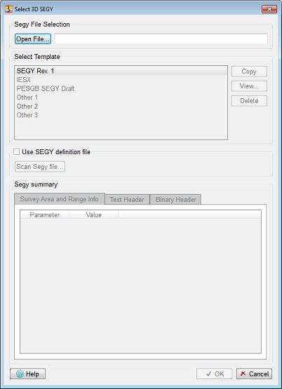
The Select SEGY Volume dialog provides you with a 3D SEGY file selector. From here you select the 3D SEGY file you require for your Stack Ghost Suppression (SGS) analysis and operator design. Unfortunately, selecting a 3D SEGY file for input here is not the end of the story. You need to also either select or build an offset mapping template for use with the selected SEGY file. Fortunately, within the software this is a straightforward task.

Figure 4.26. Select SEGY

...

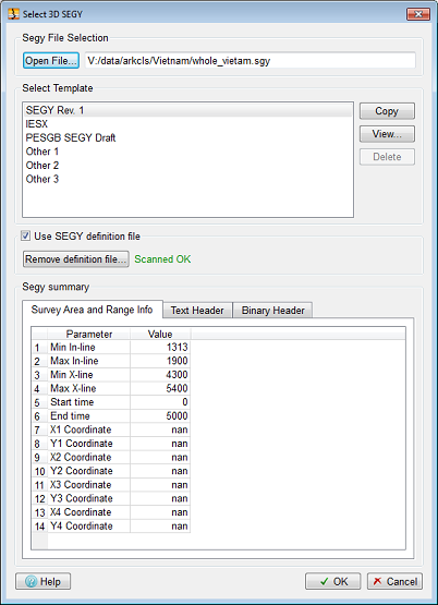
The images in the figure above show examples of the "Select SEGY" dialog for selection of SEGY files and offset mapping. The LH image shows the dialog prior to opening a SEGY file. To open a SEGY file click the Open File... push button which will pop-up a file selector dialog allowing you to traverse the file system to select and open a SEGY file. The RH image shows that a SEGY file has been opened and has been matched with an offset Template. In this case, it was matched with the "Other 1" template. This dialog attempts to automatically match the opened SEGY file with one of the available templates. If the match is successful then the matched template will be highlighted and Min/Max Inline/Xline together with Start/End Time obtained from the Opened SEGY file will be displayed in the "Survey Area and Range Info" tab within the "Segy Summary" block. Similarly the opened SEGY file's EBCDIC header information will be displayed in the "Text Header" tab with the SEGY Binary header information being displayed in the "Binary Header" tab.

Now, if no template match is found then it will be necessary to create a new template. Fortunately, this is a relatively simple process and is achieved in the following manner. Select an existing template, it doesn't really matter which one you use, then click the Copy push button. Now select the new template which will appear at the end of the list of templates and will have a default name similar to "New Template 1". Finally click Edit... push button to pop up "Edit Template" dialog. Note that existing standard templates cannot be edited (OK button is greyed out), so make a copy first.

The Edit SEGY Template dialog provides you with a mechanism to edit SEGY templates. The original SEGY standard (rev 0) has been used extensively within the oil and gas industry as a convenient way to exchange seismic data between various companies. This standard was published in 1975 for storage of 2D line seismic data on magnetic tapes. Since this original publication there have been many advancements in geophysical data acquisition including disc recording and 3D seismic. The SEGY standard was subsequently used in ways that were never originally envisioned. Inevitably, this led to inconsistent use of the trace header attributes by different companies for storage of 3D seismic on disc. Whilst the SEGY standard (rev 1) published in 2002 was designed to address such issues, there is still a need to map (set up offsets) various trace header attributes as there is software and old SEGY files in existence that don't adhere to the new SEGY rev 1 standard.

Figure 4.27. Edit Template

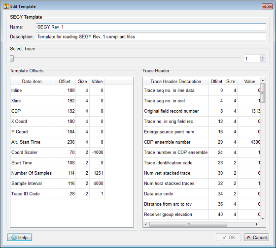
The figure above shows the "Edit Template" dialog. This dialog allows you to assign a unique name and add a brief description. The main purpose of this editor is to allow you to set up the Template Offsets for mapping various trace attributes.

OK, let's look at how we set up the various Template Offsets. This dialog works with the opened SEGY file. Within the "Select Trace" block there is a slider and a spin box object. Both allow you to move to different traces within the SEGY file. Using these objects you can position the trace reader to any trace within the SEGY file. So for any trace you will be able to display the trace header data in the right panel beneath "Trace Header" label. By scanning the trace header for a given SEGY trace you should be able to determine where in the header various pieces of information are stored. So to edit the template offset we do the following:

Whilst ARK CLS recommends that when creating a new template all data items are mapped, it may be possible to generate a template without mapping every data item in the template offset list. We consider the most important items are "Inline", "Xline", "X Coord", "Y Coord", "Coord Scaler", "Start Time", "Number Of Sample", "Sample Interval" and "Trace ID Code". These "Data Items" in the "Template Offsets" list should always be set.

The Horizon Input Dialog provides you with a horizon selector. Using the Blue Arrow select the desired horizon from Petrel.

Figure 4.28. Select Horizon

The image above shows an example of the "Select Horizon" dialog for selection of a seismic horizon.